4.2 Data Patterns and terminology
Basically the data is assumed to consist of up to four components, that is:
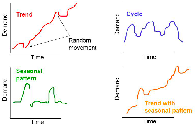
- Trend
- Long-term change in the level of data
- Positive vs. negative trends
- Stationary series have no trend
- Example: Increasing technology leading to increase in productivity
- Seasonal
- Repeated regular variation the level of data
- Example: Number of tourists in Mallorca
- Cyclical
- Wavelike upward and downward movements around the long-term trend
- Longer duration than seasonal fluctuations
- Example: Business cycles
- Note, this is very often to identify
- Irregular
- Random fluctuations
- Possibly carrying more dynamics than just deterministic ones
- Hardest to capture in a forecasting model
The four components may look similar to this:

Figure 4.2: Components in a timeseries
4.2.1 Terminology
\(Y_t\): Denotes a time series variable
\(\hat{Y_t}\): Denotes the foretasted value of \(Y_t\)
\(e_t=Y_t-\hat{Y_t}\): Denotes the residual or the forecast error.
\(Y_{t-k}\): Denotes a time series variable lagged by k periods.
4.2.1.1 Autocorrelation
Autocorrelation: is the correlation between a time series and its past (lagged) observations. To identify this, one can merely compare the lagged values as a series for itself, hence comparing actual time series against the lagged time series. This can be written as:
\[r_k=\frac{\sum_{t=k+1}^n\left(Y_{t\ }-\hat{Y}\right)}{\sum_{t=1}^n\left(Y_t-\hat{Y}\right)^{^2}}\]
Where \(k = 0,1,2,...\), hence take on numbers, typically whole numbers, as the result must be measurable.
We assess autocorrelation to identify if the data have a trend, seasons, cycles or it is random? If we have seasons, trends or cycles, we must make the model account for this, otherwise one is prone to have a model where it is just implicitly correlated, but that is merely due to the autocorrelation, as it says in the word, it is automatically correlated, but that also implies, that it is not necessarily caused by the data, but rather other factors, often we see macro factors, that have an influence, e.g. an economic book.
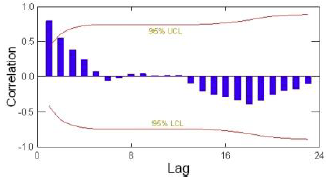
Autocorrelation can be plotted using an autocorrelation function (ACF) or merely by using a correlogram, which is a k-period plot of the autocorelation, that looks like the following:

Figure 4.3: Correlogram Example
Where one wants to be within the upper and lower level.
Manually testing for autocorrelation
One must:
- Calculate \(r_k\)
- Calculate \(SE(r_k)\)
- Hypothesis: \(H0 : \rho=0\), \(H0 : \rho≠0\)
- We apply t-test
Where: \[SE\left(r_k\right)=\sqrt{\left\{\frac{1+2\sum_{i=1}^{k-1}r_i^2}{n}\right\}}\] Although, with normal approximation \[SE\left(r_k\right)=\frac{1}{\sqrt{n-k}}\]
and test statistic equal \[t=\frac{r_k}{SE(r_k)}\]
Thence one merely must look up the cut off values and assess if there is statistical evidance for autocorrelation or not.
Alternative: Ljung-Box Q statistic
The Ljung Box Q is to identify if at least one of the components explains the Y. Thence H0 = p1 = p2 = p3 = pm, thence we want to reject this one. If not, then none of the predictors explain the Y, thus they are irregular components.
\[Q\ =\ n\left(n+2\right)\sum_{k=1}^m\frac{r_k^2}{n-k}\]
Where m is the number of lags to be tested.
The Q statistic is commonly used for testing correlation in the residuals of a forecast model and the comparison is mate to \(X^2_{m-q}\), where q is the number of parameters in the model.
4.2.1.3 Stationary vs. non stationary data
Stationary series is not trending, where is non stationary series is trending, can both be linear or exponential.
The how is it solved?
One can merely apply differencing of order k. That is equal to:
\[\Delta Y_t=Y_t-Y_{t-1}\]
One could also apply growth rates are log differencing instead.