7.6 Exercises - ADL

7.6.1 GDP and CO2 levels

df <- read_excel("Data/Week48/GDP_CO2.xls")
y <- df$co2
x <- df$gdp

Now the data is loaded and we have defined the y and x variable, being CO2 levels and GDP.

Now we can make the ADL with the following:

adl.mod <- auto_ardl(y ~ x
                     ,data = cbind(x, y) #We want to combine the variables into 1 df
                     ,max_order = 10 #Mandatory, could be other orders as well
                     ,selection = "AIC"
                     )
adl.mod <- adl.mod$best_model
adl.mod$order

## [1]  1 10

We see that according to AIC, using up to 10 lags, the optimal constellation is with 1 lag for the y variable and including 10 lags from the x variable (the additional explanatory variable)

We can assess the model that we achieved, by calling the summary.

summary(adl.mod)

## 
## Time series regression with "ts" data:
## Start = 11, End = 196
## 
## Call:
## dynlm::dynlm(formula = full_formula, data = data, start = start, 
##     end = end)
## 
## Residuals:
##      Min       1Q   Median       3Q      Max 
## -11.4432  -0.8233  -0.2912   0.9513  14.4389 
## 
## Coefficients:
##             Estimate Std. Error t value             Pr(>|t|)    
## (Intercept)  0.20914    0.32287   0.648              0.51800    
## L(y, 1)      0.82598    0.03581  23.063 < 0.0000000000000002 ***
## x            0.35123    0.06799   5.166          0.000000653 ***
## L(x, 1)     -0.24174    0.12054  -2.005              0.04648 *  
## L(x, 2)     -0.05738    0.12814  -0.448              0.65486    
## L(x, 3)     -0.08188    0.13565  -0.604              0.54690    
## L(x, 4)      0.35590    0.13428   2.650              0.00879 ** 
## L(x, 5)     -0.30012    0.13519  -2.220              0.02771 *  
## L(x, 6)      0.08400    0.13591   0.618              0.53733    
## L(x, 7)      0.20019    0.13657   1.466              0.14449    
## L(x, 8)     -0.42832    0.13544  -3.162              0.00185 ** 
## L(x, 9)      0.38239    0.13279   2.880              0.00448 ** 
## L(x, 10)    -0.26598    0.08769  -3.033              0.00279 ** 
## ---
## Signif. codes:  0 '***' 0.001 '**' 0.01 '*' 0.05 '.' 0.1 ' ' 1
## 
## Residual standard error: 3.302 on 173 degrees of freedom
## Multiple R-squared:  0.9831, Adjusted R-squared:  0.9819 
## F-statistic: 836.7 on 12 and 173 DF,  p-value: < 0.00000000000000022

We see that some of the lags appaer not to be statistically significant, although, the model is estimated to be optimized to low risk, thus we assume that the model is sufficient.

rm(list = ls())

7.6.2 Short- and long-term interest rates, exchange rates

7.6.2.1 Loading data, combining time series and assessment of stationarity

First the data is loaded, we are interested in the following:

1. Short term interest rates
2. Long term interest rates
3. Exchange rates

The data is quarterly

df <- read_excel("Data/Week48/EuroMacroData.xlsx")
stn <- df$STN %>% log() %>% ts(frequency = 4)
ltn <- df$LTN %>% log() %>% ts(frequency = 4)
een <- df$EEN %>% log() %>% ts(frequency = 4)

Now we can present the acf and pacf for each variable along with the time series for each variable.

{
  tsdisplay(stn)
  tsdisplay(ltn)
  tsdisplay(een)
}

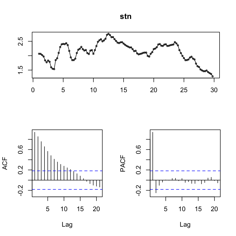
Figure 7.11: Time-Series Display

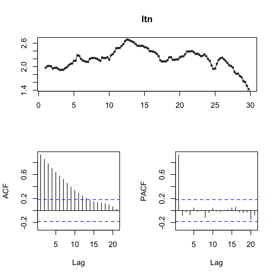
Figure 7.12: Time-Series Display

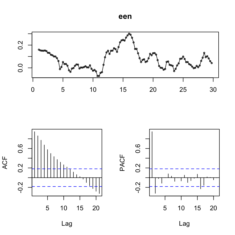
Figure 7.13: Time-Series Display

Now we are able to group the variables in one time series frame, lets denote it with z

z <- ts(cbind(stn,ltn,een), frequency = 4)

As we observed trend in the time series (hence non stationary data), we can make first order differencing to attempt to get rid of that and get stationary data.

dz <- diff(z)

We can now plot the data to see the following result.

plot(dz)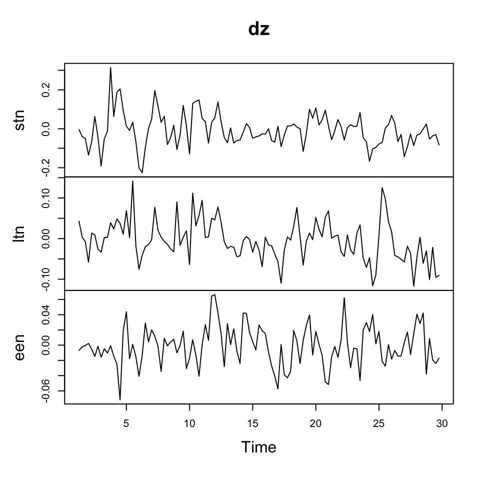

Figure 7.14: Data with 1st order differencing

Versus the raw data:

plot(z)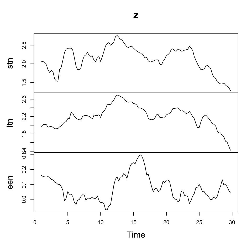

Figure 7.15: Raw data

Where we see that the changes in the observations show stationarity, where the raw data is clearly not stationary.

7.6.2.2 Vector AutoRegressive Model (VAR)

7.6.2.2.1 1. Determine order of lags to be included + model estimation

We apply VARselect(), which returns the following:

• selection: Vector with the optimal lag number according to each criterium.
• criteria: A matrix containing the values of the criteria up to lag.max.

We are only interested in finding the optimal amount of lags, p for the VAR. Hence we apply [[“selection”]]

VARselect(y = dz
          ,lag.max = 10
          ,type = "const")[["selection"]]

## AIC(n)  HQ(n)  SC(n) FPE(n) 
##      1      1      1      1

We see that the optimal amount fo lags to be included are 1. Fortunately this goes for all of the information criteria.

Hence, we have the following setting \(VAR(1)\)

Now can estimate the model, using the lag order, that we just found.

var1 <- VAR(y = dz
            ,p = 1 #How many lags to be included in the models, e.g., if p = 3,
                   # then three lags of each variable is included.
            ,type = "const")
summary(var1)

## 
## VAR Estimation Results:
## ========================= 
## Endogenous variables: stn, ltn, een 
## Deterministic variables: const 
## Sample size: 114 
## Log Likelihood: 609.086 
## Roots of the characteristic polynomial:
## 0.4441 0.4441 0.2423
## Call:
## VAR(y = dz, p = 1, type = "const")
## 
## 
## Estimation results for equation stn: 
## ==================================== 
## stn = stn.l1 + ltn.l1 + een.l1 + const 
## 
##         Estimate Std. Error t value Pr(>|t|)    
## stn.l1  0.395558   0.099033   3.994 0.000118 ***
## ltn.l1  0.293962   0.169757   1.732 0.086137 .  
## een.l1  0.328754   0.266664   1.233 0.220264    
## const  -0.002934   0.006924  -0.424 0.672604    
## ---
## Signif. codes:  0 '***' 0.001 '**' 0.01 '*' 0.05 '.' 0.1 ' ' 1
## 
## 
## Residual standard error: 0.07358 on 110 degrees of freedom
## Multiple R-Squared: 0.2626,  Adjusted R-squared: 0.2425 
## F-statistic: 13.06 on 3 and 110 DF,  p-value: 0.000000234 
## 
## 
## Estimation results for equation ltn: 
## ==================================== 
## ltn = stn.l1 + ltn.l1 + een.l1 + const 
## 
##         Estimate Std. Error t value Pr(>|t|)    
## stn.l1  0.055456   0.060338   0.919 0.360056    
## ltn.l1  0.386815   0.103428   3.740 0.000294 ***
## een.l1  0.241711   0.162471   1.488 0.139686    
## const  -0.003082   0.004219  -0.730 0.466653    
## ---
## Signif. codes:  0 '***' 0.001 '**' 0.01 '*' 0.05 '.' 0.1 ' ' 1
## 
## 
## Residual standard error: 0.04483 on 110 degrees of freedom
## Multiple R-Squared: 0.2046,  Adjusted R-squared: 0.1829 
## F-statistic: 9.429 on 3 and 110 DF,  p-value: 0.00001345 
## 
## 
## Estimation results for equation een: 
## ==================================== 
## een = stn.l1 + ltn.l1 + een.l1 + const 
## 
##         Estimate Std. Error t value Pr(>|t|)    
## stn.l1 -0.037006   0.033134  -1.117  0.26650    
## ltn.l1 -0.021367   0.056797  -0.376  0.70750    
## een.l1  0.322242   0.089221   3.612  0.00046 ***
## const  -0.001004   0.002317  -0.434  0.66549    
## ---
## Signif. codes:  0 '***' 0.001 '**' 0.01 '*' 0.05 '.' 0.1 ' ' 1
## 
## 
## Residual standard error: 0.02462 on 110 degrees of freedom
## Multiple R-Squared: 0.1313,  Adjusted R-squared: 0.1077 
## F-statistic: 5.544 on 3 and 110 DF,  p-value: 0.001396 
## 
## 
## 
## Covariance matrix of residuals:
##             stn         ltn         een
## stn  0.00541405  0.00156222 -0.00001442
## ltn  0.00156222  0.00200975 -0.00003693
## een -0.00001442 -0.00003693  0.00060607
## 
## Correlation matrix of residuals:
##           stn      ltn       een
## stn  1.000000  0.47360 -0.007963
## ltn  0.473599  1.00000 -0.033461
## een -0.007963 -0.03346  1.000000

We see that we get a model for each of the time-series and concludingly a covariance- and correlation matrixt of the residuals for the different models.

Looking at the different model estimations, we see that that e.g., lag 1 of ltn is significant for explaining ltn, where lag 1 of the other variables are not significant and so on.

As written in the code, if one was to insert p = 3 instead of 1, then we would merely have three lagged variables for each model, although it will still reflect the same signifances for the different variables.

Conclusion:

We are not able to explain anything with the other models, since there is statistical evidence for relationship between other lagged variables and the stn, ltn and een. Hence, we may be just as fine, just by doing an AR approach to each of the models, perhaps even just an AR(p=1)

7.6.2.2.2 2. Model diagnostics

Now we can make model diagnostics to check for autocorrelation (serial correlation).

This executes a Portmanteau test for correlation in the errors (i.e., autocorrelation, i.e., serial correlation). The null hypothesis is that there are no autocorrelation

serial.test(var1
            ,lags.pt = 10 #It is chosen to be 10, could be anything else, perhaps one could plot it
            ,type = "PT.asymptotic"
            )

## 
##  Portmanteau Test (asymptotic)
## 
## data:  Residuals of VAR object var1
## Chi-squared = 67.353, df = 81, p-value = 0.8612

As the p-value is far above the significane level, 5%, we cannot reject the null hypothesis, hence it is fair to assume, that the residuals are not serial correlated.

7.6.2.2.3 3. Response to shocks in the variables

With the following, we are able to deduce how the different variables react (respond) from shocks in the variables.

The y-axis expres the changes where the x-axis express the n steps ahead. Hence in this example it is quarters ahead.

plot(irf(var1,boot = TRUE, ci=0.95))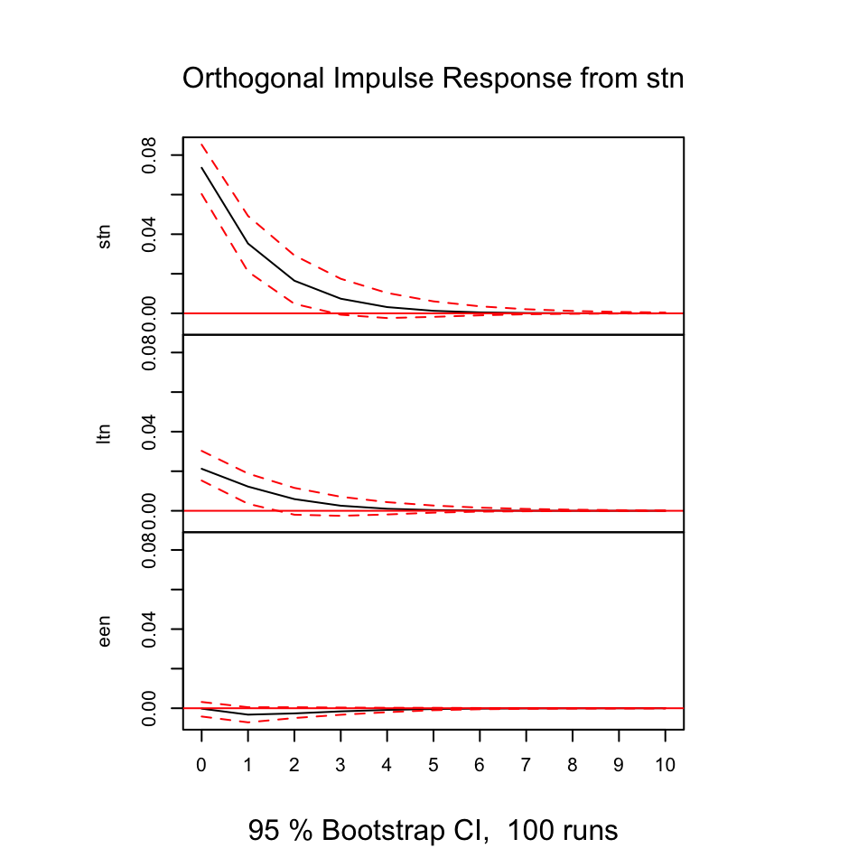

Figure 7.16: Resonses from shocks

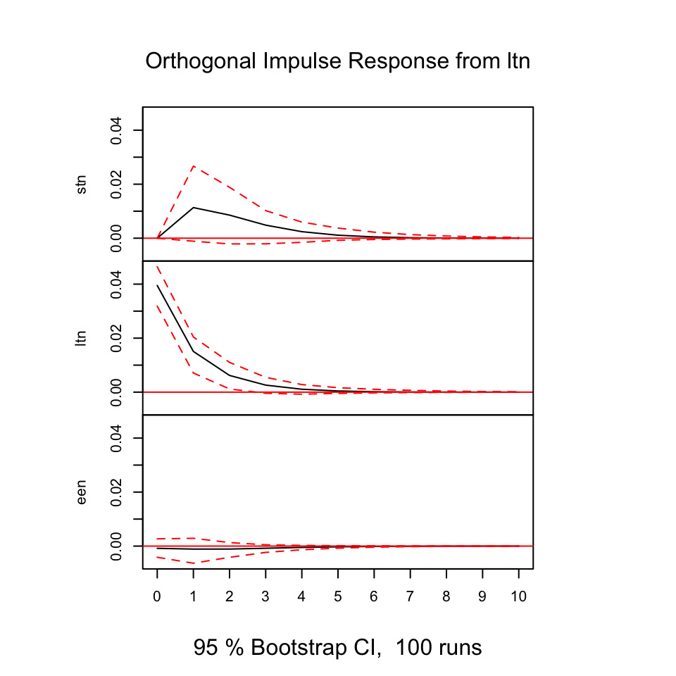
Figure 7.17: Resonses from shocks

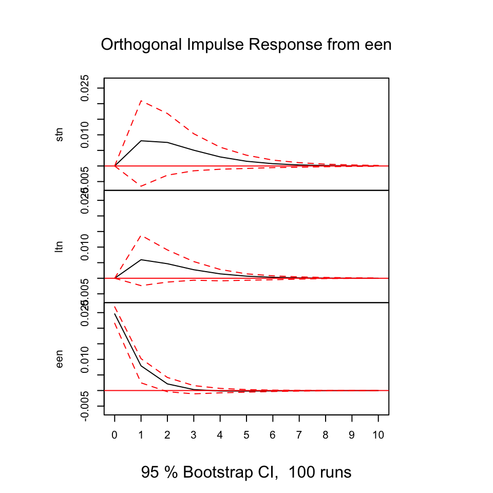
Figure 7.18: Resonses from shocks

First of all, we always see that shocks in the variables always show direct positive (same direction) response in period 0 on its own variable, that makes sens and it expected. As the illustrations above is based on models that contain one lagged period on the model, we don’t include all available information (also, it is likely that other variable explain the relationship).

E.g., looking at shocks in stn (the first figure), we see that ltn immediately tend to move in the same direction, where the effect decays over time and after some periods, it will practically be 0.

Notice, that some response have confidence intervals that are below and above 0, hence we are not really able to say how the reaction will be, same or the opposite direction.

7.6.2.2.3.1 Exogenious vs. endogenious

Terms:

• Exogenious: if a variable is extremely exogenious, it is not explain or determined by other variables
• Endogenious: if a variable is extremely endogenoius, it is explianed or determined by one or more variables.

This can be used to rank variables based on how much they are affected by other variables, with the most exogenious variable first (This is called Cholesky ordering), hence we rank based on the following principle:

lets say, that we have four variables, we want to order according to Cholesky ordering

1. Most exogenious
2. Less exogenious than 1 more than 3. Hence, more endogenious than 1. but less than 3.
3. Less exogenious than 2 more than 4. Hence, more endogenious than 2. but less than 4.
4. Most endogenious

Importance!

This is important, as it matters in the end how the forecast is done. see slides from lecture 10 page 12.

This is done by ordering according the df ‘z’ according to this.

7.6.2.2.4 4. Forecasting with ADL

This has the following steps:

1. Data partition
2. Select the order of VAR
3. Fit the model + check residuals
4. Make the forecast
5. Assessing accuracy

7.6.2.2.4.1 Step 1 - Data partition

We apply the differenced data from the exercise. The first 90 obersvations as train data and the rest test data.

insampdz <- ts(dz[1:90, 1:3], frequency = 4)
outsampdz <- dz[91:115, 1:3]

7.6.2.2.4.2 Step 2 - Select the order of VAR

We find the optimal order for p (recall VAR(p))

VARselect(insampdz
          ,lag.max = 10
          ,type="const")[["selection"]]

## AIC(n)  HQ(n)  SC(n) FPE(n) 
##      1      1      1      1

We see that the optimal order is 1.

7.6.2.2.4.3 Step 3 - Fit the model + check residuals

The data is fitted and we call the summary.

fit <- VAR(y = insampdz #The train data
           ,p = 1 #Found in step 2
           ,type="const")
summary(fit)

## 
## VAR Estimation Results:
## ========================= 
## Endogenous variables: stn, ltn, een 
## Deterministic variables: const 
## Sample size: 89 
## Log Likelihood: 480.864 
## Roots of the characteristic polynomial:
## 0.4301 0.4301 0.07976
## Call:
## VAR(y = insampdz, p = 1, type = "const")
## 
## 
## Estimation results for equation stn: 
## ==================================== 
## stn = stn.l1 + ltn.l1 + een.l1 + const 
## 
##        Estimate Std. Error t value Pr(>|t|)    
## stn.l1 0.424194   0.120074   3.533 0.000668 ***
## ltn.l1 0.098362   0.246167   0.400 0.690471    
## een.l1 0.330675   0.322101   1.027 0.307513    
## const  0.003247   0.008455   0.384 0.701865    
## ---
## Signif. codes:  0 '***' 0.001 '**' 0.01 '*' 0.05 '.' 0.1 ' ' 1
## 
## 
## Residual standard error: 0.07931 on 85 degrees of freedom
## Multiple R-Squared: 0.2173,  Adjusted R-squared: 0.1896 
## F-statistic: 7.865 on 3 and 85 DF,  p-value: 0.0001082 
## 
## 
## Estimation results for equation ltn: 
## ==================================== 
## ltn = stn.l1 + ltn.l1 + een.l1 + const 
## 
##        Estimate Std. Error t value Pr(>|t|)  
## stn.l1 0.127202   0.061310   2.075    0.041 *
## ltn.l1 0.114150   0.125692   0.908    0.366  
## een.l1 0.217023   0.164464   1.320    0.191  
## const  0.002846   0.004317   0.659    0.512  
## ---
## Signif. codes:  0 '***' 0.001 '**' 0.01 '*' 0.05 '.' 0.1 ' ' 1
## 
## 
## Residual standard error: 0.0405 on 85 degrees of freedom
## Multiple R-Squared: 0.1384,  Adjusted R-squared: 0.108 
## F-statistic: 4.552 on 3 and 85 DF,  p-value: 0.005238 
## 
## 
## Estimation results for equation een: 
## ==================================== 
## een = stn.l1 + ltn.l1 + een.l1 + const 
## 
##         Estimate Std. Error t value Pr(>|t|)    
## stn.l1 -0.038702   0.038097  -1.016 0.312572    
## ltn.l1 -0.017703   0.078103  -0.227 0.821230    
## een.l1  0.368552   0.102195   3.606 0.000523 ***
## const  -0.001251   0.002682  -0.466 0.642070    
## ---
## Signif. codes:  0 '***' 0.001 '**' 0.01 '*' 0.05 '.' 0.1 ' ' 1
## 
## 
## Residual standard error: 0.02516 on 85 degrees of freedom
## Multiple R-Squared: 0.1488,  Adjusted R-squared: 0.1187 
## F-statistic: 4.952 on 3 and 85 DF,  p-value: 0.003233 
## 
## 
## 
## Covariance matrix of residuals:
##            stn        ltn        een
## stn 0.00629028 0.00169606 0.00007265
## ltn 0.00169606 0.00163993 0.00009076
## een 0.00007265 0.00009076 0.00063321
## 
## Correlation matrix of residuals:
##        stn     ltn     een
## stn 1.0000 0.52807 0.03640
## ltn 0.5281 1.00000 0.08907
## een 0.0364 0.08907 1.00000

We see that there is not really any significant relationship between the different variables and only the lagged values of its own variable appear to be significant.

Now we can check the residuals for independency (not having serial correlation, i.e., autocorrelation). The null hypothesis is, that there is no autocorrelation.

serial.test(fit, lags.pt=10, type="PT.asymptotic")

## 
##  Portmanteau Test (asymptotic)
## 
## data:  Residuals of VAR object fit
## Chi-squared = 78.356, df = 81, p-value = 0.5626

We see the p-value being insignificant, hence we cannot reject H0 and it is fair to asume no autocorrelation.

7.6.2.2.4.4 Step 4 - Make the forecast

We apply the forecast() function to forecast the coming periods

fcast <- forecast(object = fit
                  ,h = 25) #Forecasting 25 quarters
plot(fcast)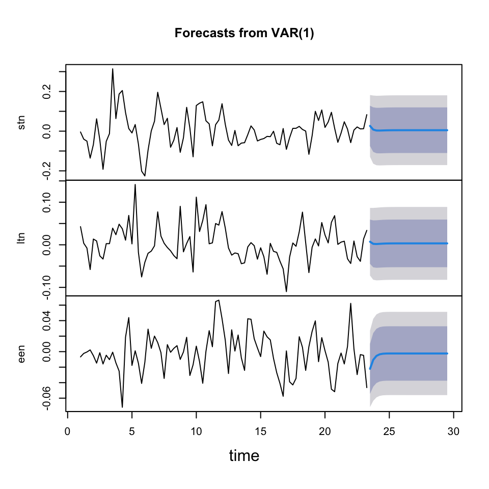

We see the forecast having a very wide confidence interval and barely any movements after a couple of periods.

This indicates that it is a bit random how it moves. If we had more seasonality, trends and cycles, then it would be easier to forecast coming periods.

7.6.2.2.4.5 Step 5 - Assessing accuracy

Now we can assess accuracy of the forecasts

accuracy(object = fcast$forecast$stn
         ,x = outsampdz[1:25,1]) #1 for stn

##                                       ME       RMSE        MAE       MPE
## Training set  0.000000000000000001407026 0.07750849 0.05654433  39.17323
## Test set     -0.053153958986903539207791 0.07534233 0.06293134 123.55935
##                  MAPE      MASE       ACF1
## Training set 174.2171 0.8031345 0.03369461
## Test set     127.4491 0.8938532         NA

accuracy(object = fcast$forecast$ltn
         ,x = outsampdz[1:25,2])

##                                       ME       RMSE        MAE      MPE
## Training set -0.000000000000000001562976 0.03957558 0.02879253 76.29913
## Test set     -0.038925425000674265807454 0.07048620 0.06082491 98.73445
##                   MAPE      MASE        ACF1
## Training set 155.66489 0.7635219 -0.03261785
## Test set      98.73445 1.6129583          NA

accuracy(object = fcast$forecast$een
         ,x = outsampdz[1:25,3])

##                                        ME       RMSE        MAE      MPE
## Training set -0.0000000000000000006126428 0.02459171 0.01934306 111.6867
## Test set      0.0064823603697087804620391 0.02516587 0.02148333 127.4315
##                  MAPE      MASE       ACF1
## Training set 221.2635 0.8012928 0.03654264
## Test set     127.4315 0.8899542         NA

We see that the MAPE is close 100% or more than 100% on average. Hence the models are not performing well. That is also expected as we see the forecasts confidence intervals are very wide and not moving much.

Even though all models are bad, it appears as if we are best at estimating ltn.