10.1 Exam 2018
df1 <- read_excel("Data/Exams/Exam2018Case1.xlsx") #Case 1 material
df2 <- read_excel("Data/Exams/Exam2018Case2.xlsx") #Case 2 material
10.1.1 Case 1
Loading the data as a time series. The series are yearly starting from 1960 and ending in 2000
ts <- ts(df1,frequency = 1,start = 1960)10.1.1.1 Q1
1. Determine the key dynamic properties of each of the series.
{tsdisplay(ts[,1],main = "Short rates") #Short term rates
tsdisplay(ts[,2],main = "Medium rates") #Medium rates
tsdisplay(ts[,3],main = "Long rates")} #Long rates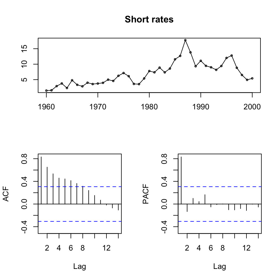
Figure 10.1: ts display of the time series
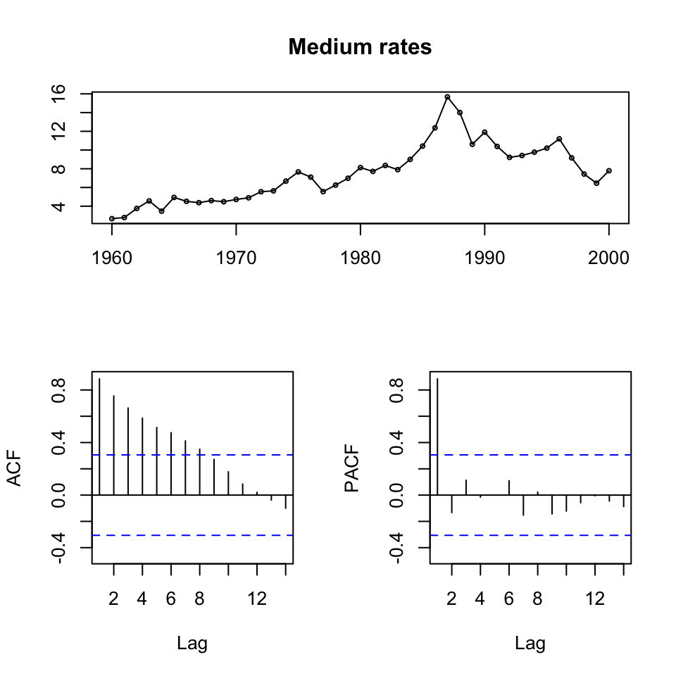
Figure 10.2: ts display of the time series
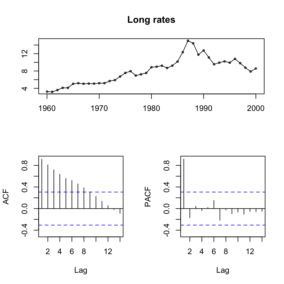
Figure 10.3: ts display of the time series
We see that all series are non stationary, hence unit roots. Also it appears as if there is a trend, an clearly if one is looking at the first 20 years, then it is quite linear.
10.1.1.2 Q2
2. Justify a model specification for Long Rates (LR) and study post-regression residuals. Obtain forecasts for LR for the period 1991-2000 based on the in-sample period 1960-1990. How does your forecast compare to a simple moving average method? Finally, obtain a forecast also for the next 18 years (2001-2018) based on 1960-2000 data.
A time series if the long term rates are is made and the the data is partitioned.
y.ltn.train <- ts[c(1:31),3] %>% ts(frequency = 1,start = 1960)
y.ltn.test <- ts[c(32:41),3]
tsdisplay(diff(y.ltn.train,1))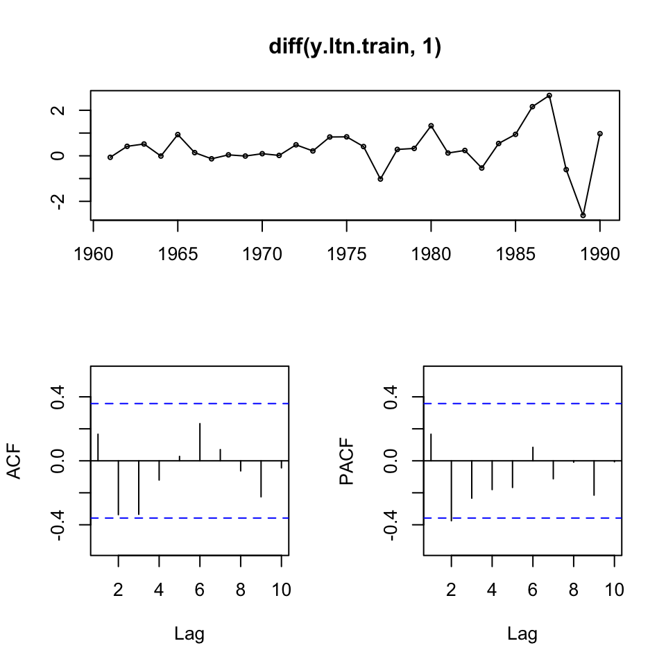
Figure 10.4: ltn inspection
We see no significant spikes, hence implying a random walk.
We saw earlier that the data was not stationary, hence we took first order difference. The data now look stationary, but has some extraordinary variance in the last years. Hence we can test this with an ADF, where H0: non stationarity.
adf.test(diff(y.ltn.train,1))##
## Augmented Dickey-Fuller Test
##
## data: diff(y.ltn.train, 1)
## Dickey-Fuller = -3.5238, Lag order = 3, p-value = 0.05851
## alternative hypothesis: stationaryBased on the 5% level we are not able to reject H0, but it is very close to the significance level. It was found, that H0 can be rejected with d = 2, where p value would be ≈ 0,036, hence rejecting H0 on the five percent level. Although it would make the data more abstract from the actual data.
Hence it is chosen to select the first order difference, well in mind, that it is not significant on the 5% level. But, that is also the probability of taking the wrong decision.
So seeing that we have a random walk. We can assess the men of the data, and see where it lies.
mean(diff(y.ltn.train))## [1] 0.316111We see a mean of 0,3161 indicating, that the model has a drift.
Thus we can make the following model, being an RW with a drift.
fit <- Arima(y.ltn.train,order = c(0,1,0),include.drift = TRUE)
summary(fit)
## Series: y.ltn.train
## ARIMA(0,1,0) with drift
##
## Coefficients:
## drift
## 0.3161
## s.e. 0.1652
##
## sigma^2 estimated as 0.8469: log likelihood=-39.57
## AIC=83.13 AICc=83.58 BIC=85.94
##
## Training set error measures:
## ME RMSE MAE MPE MAPE MASE
## Training set 0.00009480282 0.8900961 0.5748442 -0.8163705 6.898777 0.8854342
## ACF1
## Training set 0.1662727Now we are able to forecast
10.1.1.2.1 Forecasting using ARIMA
Forecasting
forecast(object = fit,h = 10)## Point Forecast Lo 80 Hi 80 Lo 95 Hi 95
## 1991 13.05444 11.87506 14.23382 11.25073 14.85815
## 1992 13.37055 11.70265 15.03845 10.81972 15.92138
## 1993 13.68666 11.64391 15.72941 10.56254 16.81078
## 1994 14.00277 11.64401 16.36154 10.39535 17.61020
## 1995 14.31888 11.68170 16.95607 10.28567 18.35210
## 1996 14.63500 11.74611 17.52388 10.21683 19.05317
## 1997 14.95111 11.83075 18.07146 10.17894 19.72328
## 1998 15.26722 11.93142 18.60302 10.16555 20.36888
## 1999 15.58333 12.04518 19.12148 10.17220 20.99446
## 2000 15.89944 12.16990 19.62898 10.19561 21.60327forecast.test <- Arima(y = ts[,3] #The ltn
,model = fit) #We apply the model that was found above, hence 0,1,0 + drift
knitr::kable(t(t(forecast.test$fitted[c(32:41)])),caption = "Fitted values test period")| 13.054441 |
| 11.430281 |
| 9.860281 |
| 10.242781 |
| 10.543611 |
| 10.237781 |
| 11.127781 |
| 10.122781 |
| 9.087781 |
| 8.192781 |
Now we can calculate accuracy
accuracy(object = forecast.test$fitted[c(32:41)],x = y.ltn.test)## ME RMSE MAE MPE MAPE
## Test set -0.731944 1.150236 0.9374434 -7.739819 9.837796We see that we get an RMSE of 1.15 and MPE of -7.7
10.1.1.2.2 Forecasting with simple moving averages 1991 - 2000
Calculating simple moving average
We know that the data is not stationary, hence we must make differencing.
y.ltn <- ts(ts[,3],start = 1960)
dy.ltn <- diff(y.ltn)
dy.ltn.test <- dy.ltn[31:40]
ma.ltn <- ma(x = dy.ltn,order = 3)
plot(ma.ltn) + grid(col = "lightgrey")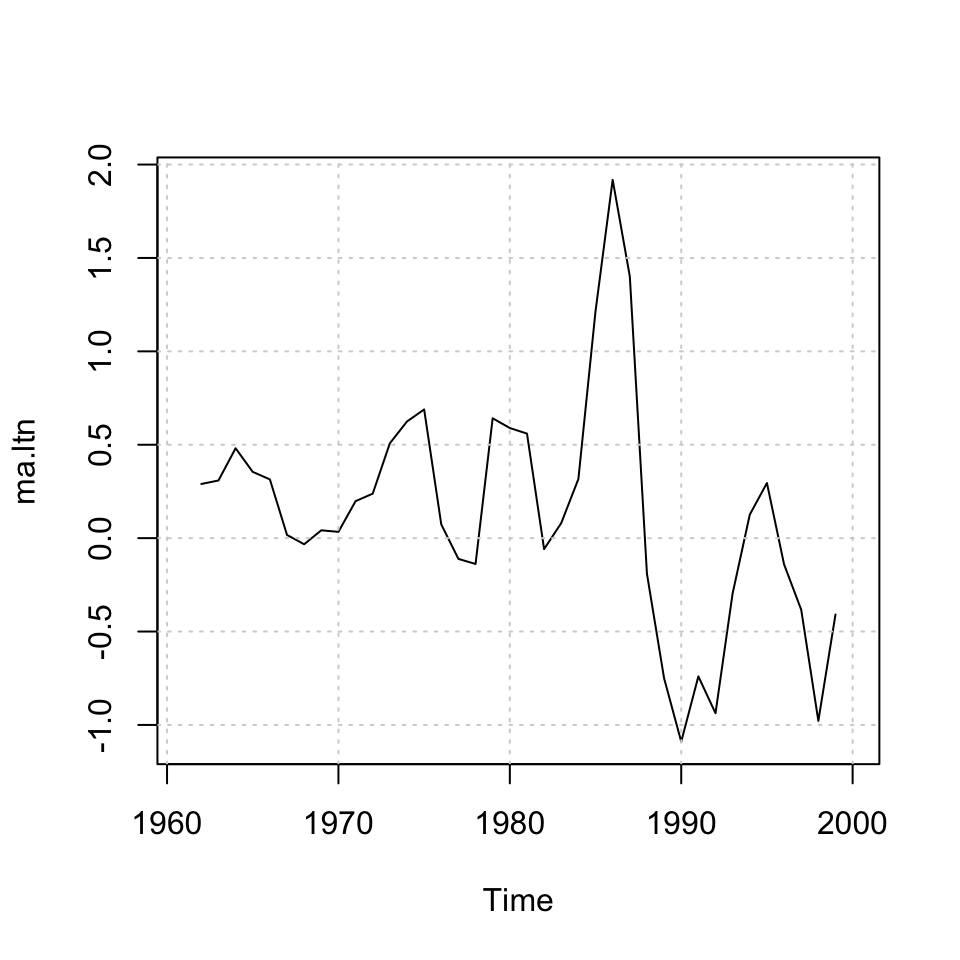
## integer(0)We see the MA’s above.
We see that the MA’s are centered, that is not applicable for prediction purposes, as we want to predict using previous periods.
FORECASTING WITH MA
It is done with three different approaches:
- Using
ma()not really good - Using excel and importing, that is valid
- Using some loops, that is pretty cool
10.1.1.2.2.1 1. Using ma()
USING MA
This is not really applicable for forecasting.
k <- 3 #specify the order of the moving average
c <- rep (1/k,k) #remember that simple average is a weighted average with equal weights,
                #you need to specify weights for the filter command to work

#Applying filter, to move the MA's to the end of the period
yt3 <- stats::filter(x = dy.ltn #The time-series
                     ,filter = c #The filter (the wheights)
                     ,sides = 1)

#Plotting
ts.plot(yt3) + grid(col = "Lightgrey") #Plotting the MA's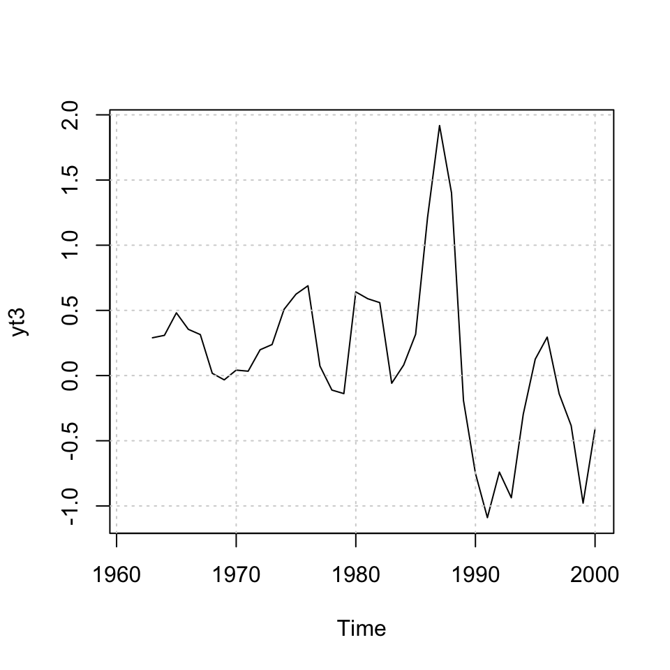
Figure 10.5: MA ltn data
## integer(0)Then one could make accuracy
10.1.1.2.2.2 2. Using excel
Doing it in excel and then importing
temp <- read_excel("Data/temp.xlsx")
ma3.excel <- temp[,3]
ma3.excel <- ts(ma3.excel)
accuracy
ma.forecast.test <- yt3[c(32:41)]
accuracy(object = ma3.excel,x = dy.ltn.test)
## ME RMSE MAE MPE MAPE
## Test set -0.568935 1.061947 0.991435 129.1631 129.163110.1.1.2.2.3 3. Using a loop
Using a loop for this purpose
#Define the input data
dy.ltn.train <- dy.ltn[1:30]
dy.ltn.test <- dy.ltn[31:40]

#Forecasting with a simple MA of order k
k <- 3
l <- length(dy.ltn.train) #number of available data points

#adding extra rows, as many as periods ahead want to forecast
h <-10
y <- dy.ltn.train

#generating space to save the forecasts
for (i in 1:h){
  y <- c(y, 0)
}
t(t(y))
## [,1]
## [1,] -0.06583
## [2,] 0.41666
## [3,] 0.51917
## [4,] -0.01000
## [5,] 0.93417
## [6,] 0.14000
## [7,] -0.13084
## [8,] 0.04250
## [9,] -0.01000
## [10,] 0.09334
## [11,] 0.01750
## [12,] 0.48333
## [13,] 0.21333
## [14,] 0.82667
## [15,] 0.83333
## [16,] 0.40667
## [17,] -1.02000
## [18,] 0.28000
## [19,] 0.32500
## [20,] 1.32000
## [21,] 0.12333
## [22,] 0.23584
## [23,] -0.53584
## [24,] 0.54250
## [25,] 0.94334
## [26,] 2.15916
## [27,] 2.65084
## [28,] -0.60584
## [29,] -2.61833
## [30,] 0.97333
## [31,] 0.00000
## [32,] 0.00000
## [33,] 0.00000
## [34,] 0.00000
## [35,] 0.00000
## [36,] 0.00000
## [37,] 0.00000
## [38,] 0.00000
## [39,] 0.00000
## [40,] 0.00000Now we see that we have extended the ts with 10 rows of 0. Corresponding with the period that we want to forecast.
Now we can do the forecast
#calculating the forecast values
for (j in (l+1):(l+h)){
  a<-j-k
  b<-j-1
  x <-y[a:b]
  y[j] <- mean(x)
}
t(t(y))
## [,1]
## [1,] -0.0658300
## [2,] 0.4166600
## [3,] 0.5191700
## [4,] -0.0100000
## [5,] 0.9341700
## [6,] 0.1400000
## [7,] -0.1308400
## [8,] 0.0425000
## [9,] -0.0100000
## [10,] 0.0933400
## [11,] 0.0175000
## [12,] 0.4833300
## [13,] 0.2133300
## [14,] 0.8266700
## [15,] 0.8333300
## [16,] 0.4066700
## [17,] -1.0200000
## [18,] 0.2800000
## [19,] 0.3250000
## [20,] 1.3200000
## [21,] 0.1233300
## [22,] 0.2358400
## [23,] -0.5358400
## [24,] 0.5425000
## [25,] 0.9433400
## [26,] 2.1591600
## [27,] 2.6508400
## [28,] -0.6058400
## [29,] -2.6183300
## [30,] 0.9733300
## [31,] -0.7502800
## [32,] -0.7984267
## [33,] -0.1917922
## [34,] -0.5801663
## [35,] -0.5234617
## [36,] -0.4318067
## [37,] -0.5118116
## [38,] -0.4890267
## [39,] -0.4775483
## [40,] -0.4927955accuracy(object = y[(length(y)-9):(length(y))],x = dy.ltn.test)## ME RMSE MAE MPE MAPE
## Test set 0.1088786 0.8003623 0.7292919 94.18366 108.4159plot(y,type = 'l',main = "MA, k = 3") + abline(v = l,col = "red") + grid(col = "lightgrey")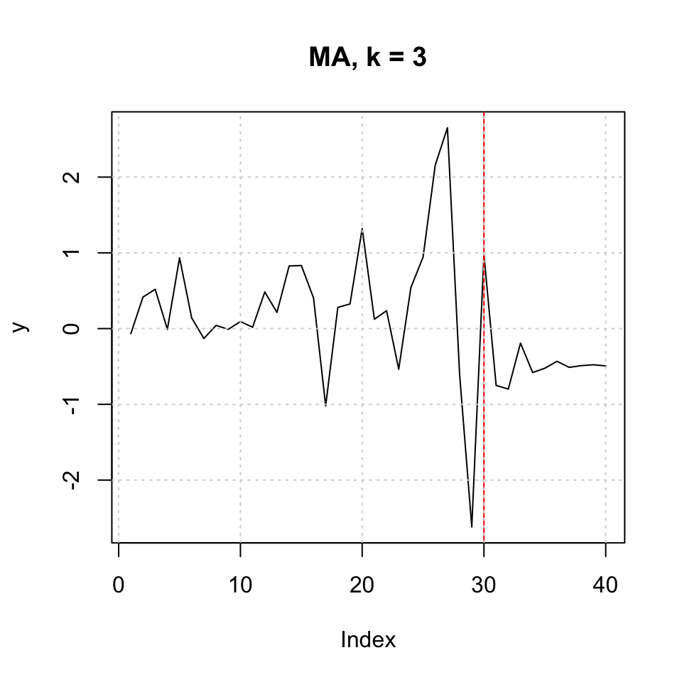
Figure 10.6: MA k=3 h=10
## integer(0)Conclusion
ARIMA RMSE = 1.15 MA3 RMSE = 0.800
Hence MA appear to be the better approach.
10.1.1.3 Forecasting 2001 - 2018
Forecasting 18 years
10.1.1.3.1 Using ma (loop method)
#Define the input data
dy.ltn <- dy.ltn

#Forecasting with a simple MA of order k
k <- 3
l <- length(dy.ltn) #number of available data points

#adding extra rows, as many as periods ahead want to forecast
h <-18
y <- dy.ltn

#generating space to save the forecasts
for (i in 1:h){
  y <- c(y, 0)
}
t(t(y))
## [,1]
## [1,] -0.06583
## [2,] 0.41666
## [3,] 0.51917
## [4,] -0.01000
## [5,] 0.93417
## [6,] 0.14000
## [7,] -0.13084
## [8,] 0.04250
## [9,] -0.01000
## [10,] 0.09334
## [11,] 0.01750
## [12,] 0.48333
## [13,] 0.21333
## [14,] 0.82667
## [15,] 0.83333
## [16,] 0.40667
## [17,] -1.02000
## [18,] 0.28000
## [19,] 0.32500
## [20,] 1.32000
## [21,] 0.12333
## [22,] 0.23584
## [23,] -0.53584
## [24,] 0.54250
## [25,] 0.94334
## [26,] 2.15916
## [27,] 2.65084
## [28,] -0.60584
## [29,] -2.61833
## [30,] 0.97333
## [31,] -1.62416
## [32,] -1.57000
## [33,] 0.38250
## [34,] 0.30083
## [35,] -0.30583
## [36,] 0.89000
## [37,] -1.00500
## [38,] -1.03500
## [39,] -0.89500
## [40,] 0.70333
## [41,] 0.00000
## [42,] 0.00000
## [43,] 0.00000
## [44,] 0.00000
## [45,] 0.00000
## [46,] 0.00000
## [47,] 0.00000
## [48,] 0.00000
## [49,] 0.00000
## [50,] 0.00000
## [51,] 0.00000
## [52,] 0.00000
## [53,] 0.00000
## [54,] 0.00000
## [55,] 0.00000
## [56,] 0.00000
## [57,] 0.00000
## [58,] 0.00000Now we see that we have extended the ts with 10 rows of 0. Corresponding with the period that we want to forecast.
Now we can do the forecast
#calculating the forecast values
for (j in (l+1):(l+h)){
  a<-j-k
  b<-j-1
  x <-y[a:b]
  y[j] <- mean(x)
}
t(t(y))
## [,1]
## [1,] -0.06583000
## [2,] 0.41666000
## [3,] 0.51917000
## [4,] -0.01000000
## [5,] 0.93417000
## [6,] 0.14000000
## [7,] -0.13084000
## [8,] 0.04250000
## [9,] -0.01000000
## [10,] 0.09334000
## [11,] 0.01750000
## [12,] 0.48333000
## [13,] 0.21333000
## [14,] 0.82667000
## [15,] 0.83333000
## [16,] 0.40667000
## [17,] -1.02000000
## [18,] 0.28000000
## [19,] 0.32500000
## [20,] 1.32000000
## [21,] 0.12333000
## [22,] 0.23584000
## [23,] -0.53584000
## [24,] 0.54250000
## [25,] 0.94334000
## [26,] 2.15916000
## [27,] 2.65084000
## [28,] -0.60584000
## [29,] -2.61833000
## [30,] 0.97333000
## [31,] -1.62416000
## [32,] -1.57000000
## [33,] 0.38250000
## [34,] 0.30083000
## [35,] -0.30583000
## [36,] 0.89000000
## [37,] -1.00500000
## [38,] -1.03500000
## [39,] -0.89500000
## [40,] 0.70333000
## [41,] -0.40889000
## [42,] -0.20018667
## [43,] 0.03141778
## [44,] -0.19255296
## [45,] -0.12044062
## [46,] -0.09385860
## [47,] -0.13561739
## [48,] -0.11663887
## [49,] -0.11537162
## [50,] -0.12254263
## [51,] -0.11818437
## [52,] -0.11869954
## [53,] -0.11980885
## [54,] -0.11889759
## [55,] -0.11913533
## [56,] -0.11928059
## [57,] -0.11910450
## [58,] -0.11917347plot(y,type = 'l',main = "MA, k = 3") + abline(v = l,col = "red") + grid(col = "lightgrey")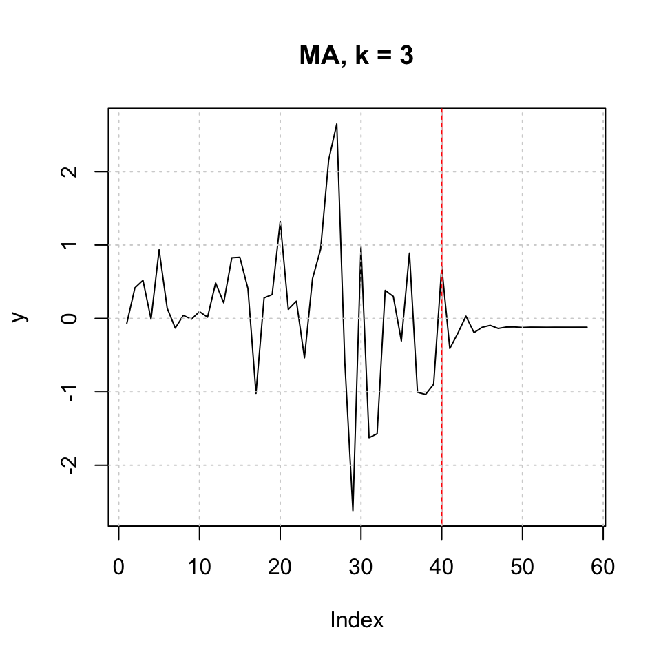
Figure 10.7: MA k=3 h=18
## integer(0)10.1.1.3.2 Using ARIMA (RW + drift)
As we have a random walk with a drift, we merely see that the forecast follow the drift, which consist of the mean of the train data set.
forecast(object = forecast.test,h = 18) %>% plot()<img src=“Business-Forecasting-Notebook_files/figure-html/fig.cap”Forecast with RW + drift“-1.png” width=“480” style=“display: block; margin: auto;” />
10.1.2 Q3
3. In a multiple regression framework, determine the relationship of LR with SR and MR. Study whether the residuals satisfy the OLS assumptions.
df1 <- read_excel("Data/Exams/Exam2018Case1.xlsx") #Case 1 material
stn <- df1[,1] %>% ts(start = 1960)
mtn <- df1[,2] %>% ts(start = 1960)
ltn <- df1[,3] %>% ts(start = 1960)

fit <- lm(ltn ~ mtn + stn)
summary(fit)
##
## Call:
## lm(formula = ltn ~ mtn + stn)
##
## Residuals:
## Min 1Q Median 3Q Max
## -0.8618 -0.2749 -0.0409 0.1577 0.9019
##
## Coefficients:
## Estimate Std. Error t value Pr(>|t|)
## (Intercept) -0.07300 0.22196 -0.329 0.744
## mtn 1.43944 0.09113 15.795 < 0.0000000000000002 ***
## stn -0.40008 0.07491 -5.341 0.00000456 ***
## ---
## Signif. codes: 0 '***' 0.001 '**' 0.01 '*' 0.05 '.' 0.1 ' ' 1
##
## Residual standard error: 0.3856 on 38 degrees of freedom
## Multiple R-squared: 0.9842, Adjusted R-squared: 0.9834
## F-statistic: 1185 on 2 and 38 DF, p-value: < 0.00000000000000022We see that there is statistical evidence for relationship between the variables.
Although we may have a concern for multicollinearity.
vif(fit)## mtn stn
## 20.91306 20.91306We see that the values far above 10, hence according to the rule of thumb, we have multicollinearity. Meaning that we should remove one of the variables, as they explain the same.
10.1.2.1 Diagnostics
10.1.2.1.1 Check for heteroskedasticity
plot(residuals(fit)) + abline(h = 0) + grid(col = "grey")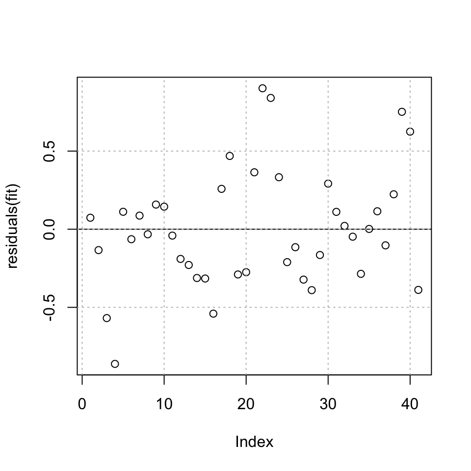
Figure 10.8: Residuals plot of the fit
## integer(0)It appears as if there can be heteroskedasticity in the residuals, meaning that there is information in the data, that is not explained by our model, hence the variance and the mean changes over time.
Although it is a good idea to make a test for this. Here a Breusch-Pagan test:
bptest(fit)##
## studentized Breusch-Pagan test
##
## data: fit
## BP = 0.27942, df = 2, p-value = 0.8696We see that there is in fact not enough evidence to reject the null, meaning it is fair to assume that the H0 is true, hence have homoskedasticity in the residuals.
10.1.2.1.2 Check for independent residuals
adf.test(resid(fit))##
## Augmented Dickey-Fuller Test
##
## data: resid(fit)
## Dickey-Fuller = -3.2478, Lag order = 3, p-value = 0.09348
## alternative hypothesis: stationaryWe reject H0, hence it is fair to assume that the residuals are non stationary, i.e. has unit root.
One could also apply Durbin-Watson test, to check for independent residuals.
10.1.2.1.3 Checking residuals for normality
Therefore, we can also plot a histogram of the data to assess the normal
We use a Jarque Bera test, where H0: Normal distribution
tseries::jarque.bera.test(resid(fit))##
## Jarque Bera Test
##
## data: resid(fit)
## X-squared = 1.5466, df = 2, p-value = 0.4615hist(resid(fit))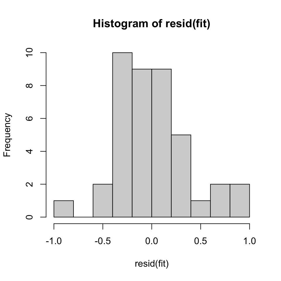
Figure 10.9: Check for normality
Based on the JB test, it is in fact normal distribution in the residuals. This can be seen from the histogram as well, although there is some small skewness.
10.1.2.1.4 Conclusion
We do not meet the requirements, as we observe the following issues:
- Multicollinearity
- Autocorrelation
10.1.3 Q4
4. If residuals from the previous regression are satisfactory, interpret the estimation output from the previous step. Otherwise, make the necessary transformations so that you obtain valid estimates, and compare how the results change.
10.1.3.1 Test without integration
We try to remove one variable to get rid of multicollinearity and then see how it affects the model.
{
  fit <- lm(ltn ~ stn)
  bptest(fit) %>% print() #Check for independent residuals
  adf.test(resid(fit)) %>% print() #Test for autocorrelation
  dwtest(fit) %>% print() #Test for autocorrelation
  jarque.bera.test(resid(fit))  %>% print() #Check for normality in the residuals
}
##
## studentized Breusch-Pagan test
##
## data: fit
## BP = 2.0956, df = 1, p-value = 0.1477
##
##
## Augmented Dickey-Fuller Test
##
## data: resid(fit)
## Dickey-Fuller = -3.8954, Lag order = 3, p-value = 0.02361
## alternative hypothesis: stationary
##
##
## Durbin-Watson test
##
## data: fit
## DW = 0.82013, p-value = 0.000006044
## alternative hypothesis: true autocorrelation is greater than 0
##
##
## Jarque Bera Test
##
## data: resid(fit)
## X-squared = 1.5021, df = 2, p-value = 0.4719We see that the ADF show no non stationarity, hence autocorrelation, but the DW does show non stationarity (hence autocorrelation)
We can check for cointegration, to see if they are in fact cointegrated, hence it is acceptable to have variables, that are not stationary. This can be check with the Phillips-Ouliaris test (2-step EG test).
z <- ts(cbind(stn,ltn))
po.test(z) #Note, this is the 2-step EG test
##
## Phillips-Ouliaris Cointegration Test
##
## data: z
## Phillips-Ouliaris demeaned = -19.899, Truncation lag parameter = 0,
## p-value = 0.05735We see that the p-value is 5.7% hence there is not sufficient evidence to reject on the five percent level, hence it is questionable.
Sub conclusion
The variables are not cointegrated, hence one should make the data series’ stationary by first order integration.
10.1.3.2 Test with first order integration
{
  fit <- lm(diff(ltn) ~ diff(stn))
  bptest(fit) %>% print() #Check for independent residuals
  adf.test(resid(fit))  %>% print() #Test for autocorrelation
  dwtest(fit)  %>% print() #Test for autocorrelation
  jarque.bera.test(resid(fit))  %>% print() #Check for normality in the residuals
}
##
## studentized Breusch-Pagan test
##
## data: fit
## BP = 0.07672, df = 1, p-value = 0.7818
##
##
## Augmented Dickey-Fuller Test
##
## data: resid(fit)
## Dickey-Fuller = -2.889, Lag order = 3, p-value = 0.2246
## alternative hypothesis: stationary
##
##
## Durbin-Watson test
##
## data: fit
## DW = 1.9979, p-value = 0.4942
## alternative hypothesis: true autocorrelation is greater than 0
##
##
## Jarque Bera Test
##
## data: resid(fit)
## X-squared = 2.8678, df = 2, p-value = 0.238410.1.4 Q5
5. Based on the valid regression you obtain in the previous step, produce an 18-year (2001-2018) forecast for LR, assuming the estimated coeficients remain the same for the 18-year duration. Compare your findings to the forecasts you obtained in step 2. Interpret what leads to the diference, if any, in the forecasts.
Skipped, hasnt done similar during the semester
10.1.5 Q6
6. Treat these three variables in a VAR setting, justifying the number of lags you use. Interpret the estimation output. Why are you getting these results? If possible, justify a Cholesky ordering, plot Impulse Responses and Forecast Error Variance Decompositions, and interpret them.
This was not really covered during lectures. we did VAR in bivariate setting
10.1.5.1 Vector AutoRegressive Model (VAR)
df1 <- read_excel("Data/Exams/Exam2018Case1.xlsx") #Case 1 material
sr <- ts(df1$SR,start = 1960)
mr <- ts(df1$MR,start = 1960)
lr <- ts(df1$LR,start = 1960)
{
tsdisplay(sr)
tsdisplay(mr)
tsdisplay(lr)
}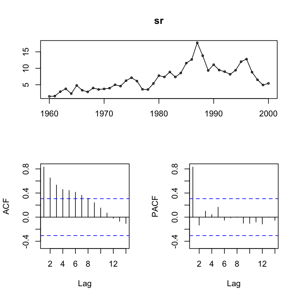
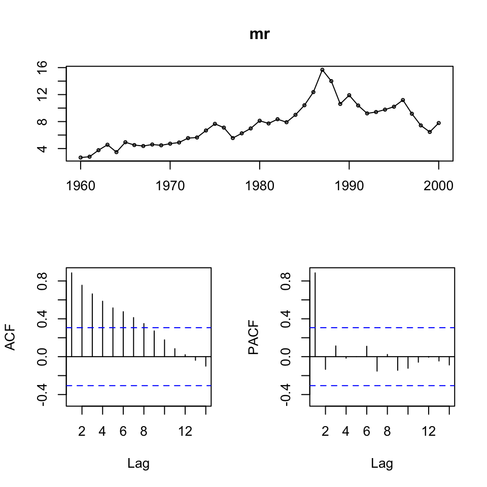
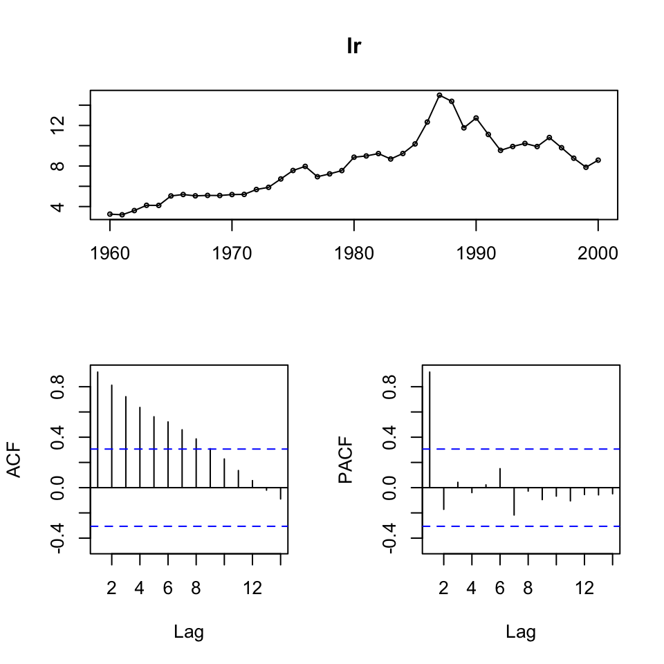
We see that the series’ are not stationary. Hence, we must do first order differencing.
dsr <- ts(df1$SR,start = 1960) %>% diff()
dmr <- ts(df1$MR,start = 1960) %>% diff()
dlr <- ts(df1$LR,start = 1960) %>% diff()

par(mfrow = c(3,1))
plot(dsr,main = "Diff. SR") + grid(col = "grey")
## integer(0)plot(dmr,main = "Diff. MR") + grid(col = "grey")## integer(0)plot(dlr,main = "Diff. LR") + grid(col = "grey")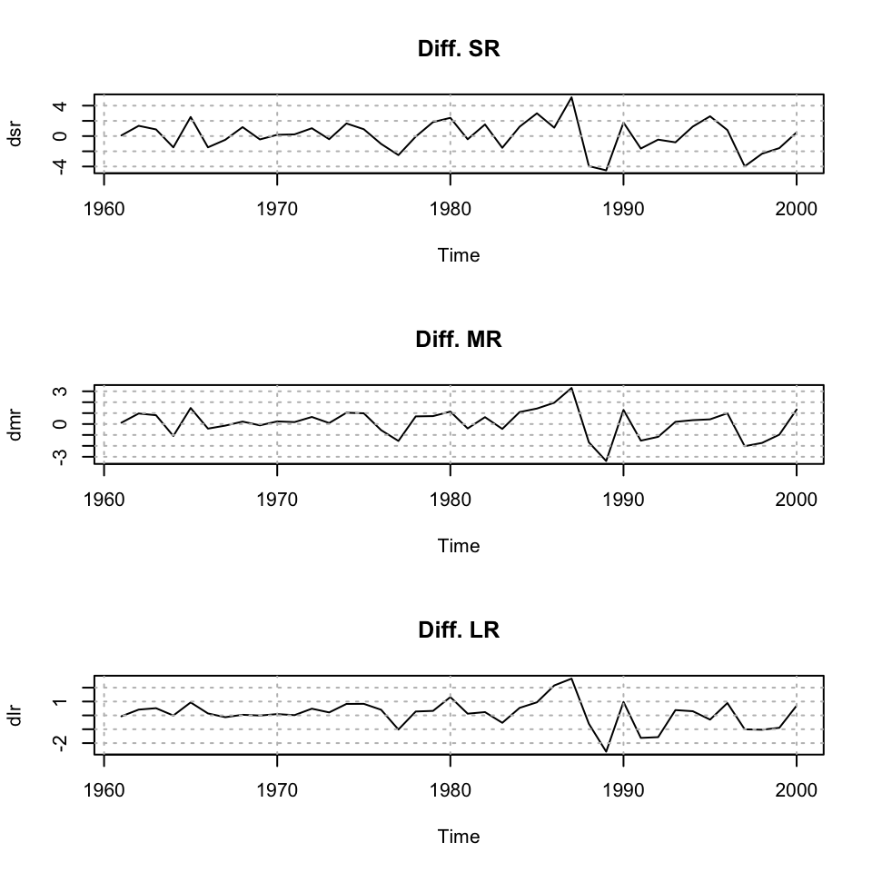
Figure 10.10: Plotting time series
## integer(0)We see that the data now appear stationary, and we are able to work with the series’
{acf(dsr)
acf(dmr)
acf(dlr)}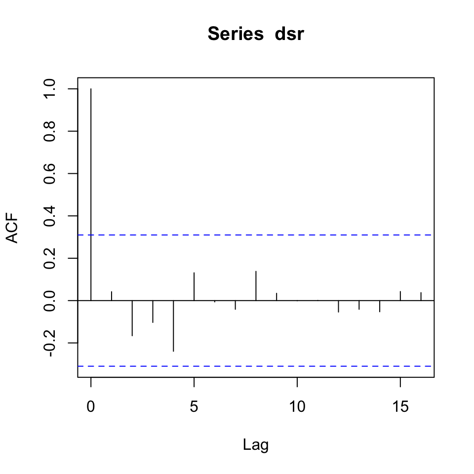
Figure 10.11: Correlogram of the series’
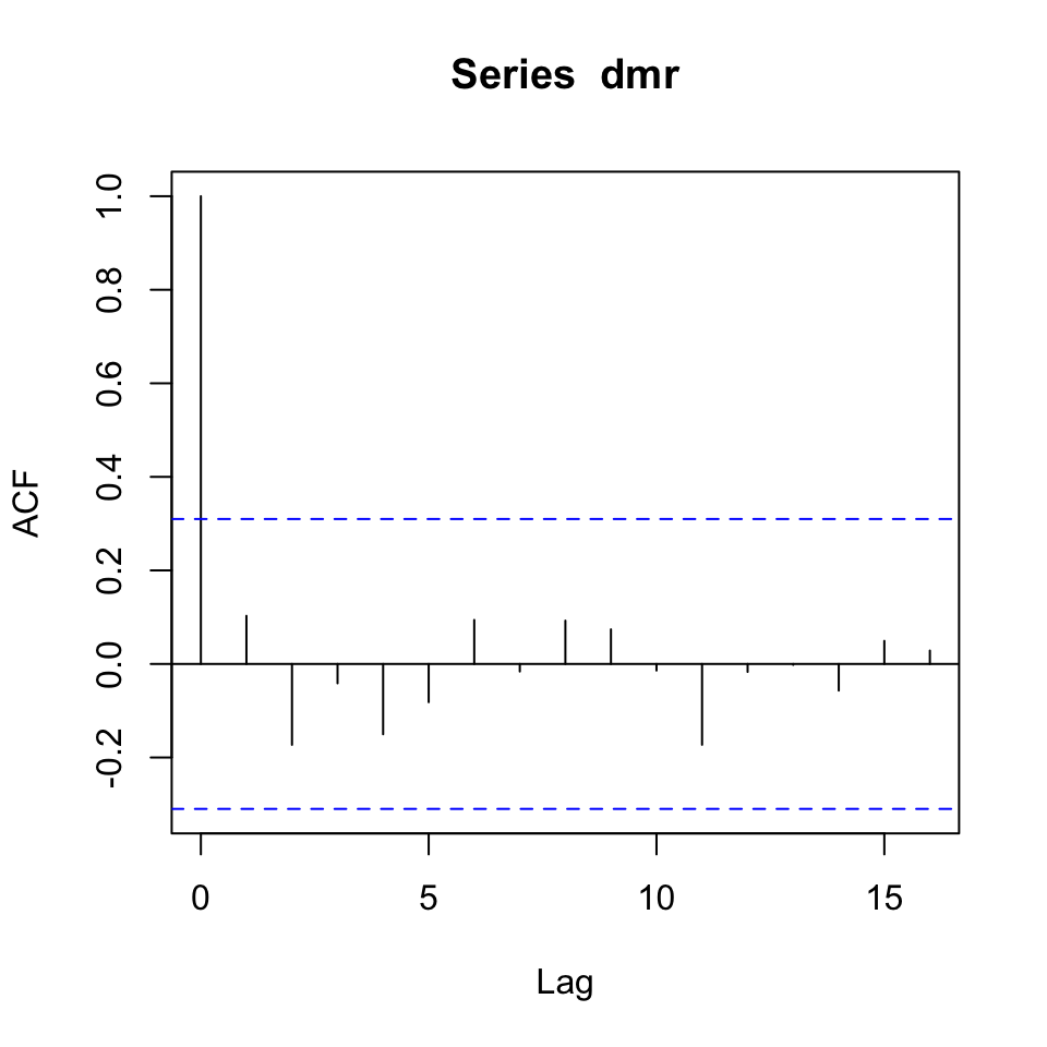
Figure 10.12: Correlogram of the series’
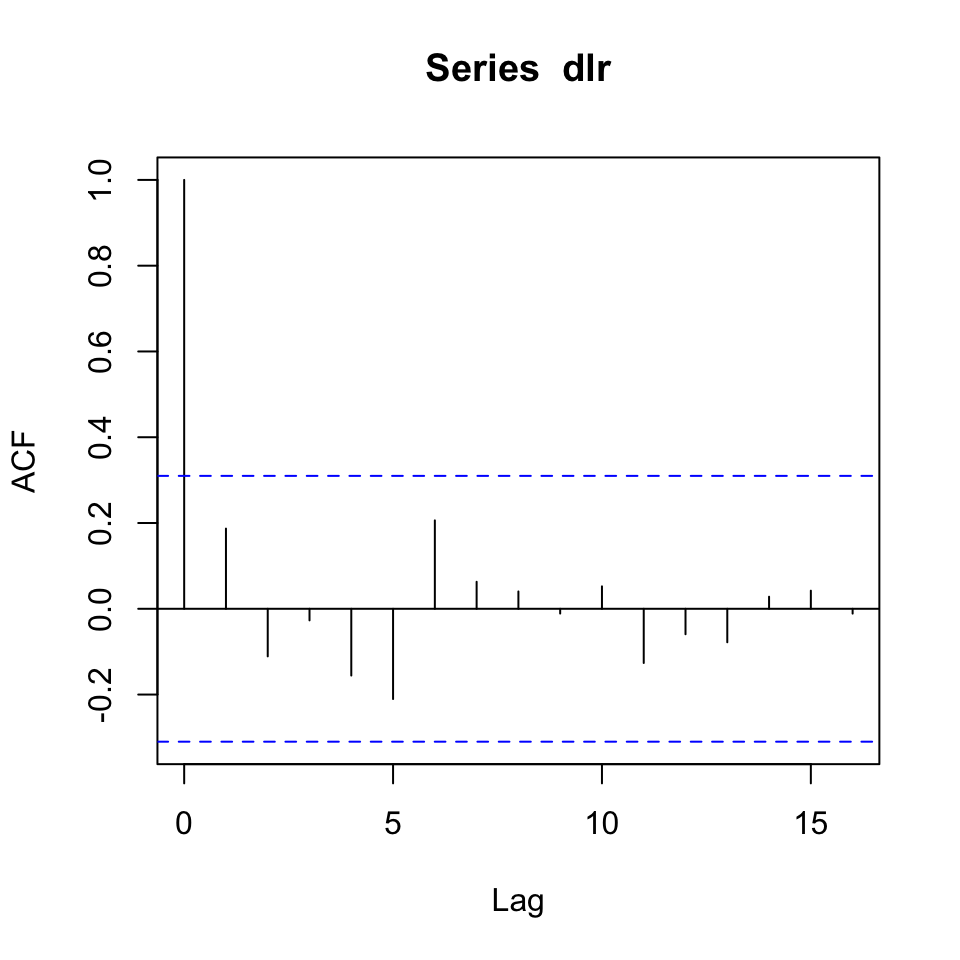
Figure 10.13: Correlogram of the series’
10.1.5.1.1 1. Determine order of lags to be included + model estimation
dz <- ts(cbind(sr,mr,lr),start = 1960) #dz = differenced z, where z equal the dataframe
dz <- diff(dz)
VARselect(y = dz
          ,lag.max = 5 #if = 10, then AIC becomes -Inf, then it will select that, although that is faulty
          ,type = "const")
## $selection
## AIC(n) HQ(n) SC(n) FPE(n)
## 1 1 1 1
##
## $criteria
## 1 2 3 4 5
## AIC(n) -2.1319476 -1.9610699 -1.9981813 -1.71593364 -1.5732805
## HQ(n) -1.9478656 -1.6389263 -1.5379762 -1.11766703 -0.8369524
## SC(n) -1.5986854 -1.0278611 -0.6650258 0.01716849 0.5597683
## FPE(n) 0.1189635 0.1430338 0.1424012 0.20108463 0.2582111According to all IC, we should set p = 1, hence \(VAR(p=1)\)
Now can estimate the model, using the lag order, that we just found.
var1 <- VAR(y = dz
            ,p = 1 #How many lags to be included in the models, e.g., if p = 3,
                   # then three lags of each variable is included.
            ,type = "const")
summary(var1)
##
## VAR Estimation Results:
## =========================
## Endogenous variables: sr, mr, lr
## Deterministic variables: const
## Sample size: 39
## Log Likelihood: -112.684
## Roots of the characteristic polynomial:
## 0.307 0.307 0.1904
## Call:
## VAR(y = dz, p = 1, type = "const")
##
##
## Estimation results for equation sr:
## ===================================
## sr = sr.l1 + mr.l1 + lr.l1 + const
##
## Estimate Std. Error t value Pr(>|t|)
## sr.l1 -0.1984 0.5247 -0.378 0.708
## mr.l1 1.0410 1.4028 0.742 0.463
## lr.l1 -0.9496 1.1081 -0.857 0.397
## const 0.1280 0.3363 0.381 0.706
##
##
## Residual standard error: 2.075 on 35 degrees of freedom
## Multiple R-Squared: 0.02227, Adjusted R-squared: -0.06154
## F-statistic: 0.2657 on 3 and 35 DF, p-value: 0.8497
##
##
## Estimation results for equation mr:
## ===================================
## mr = sr.l1 + mr.l1 + lr.l1 + const
##
## Estimate Std. Error t value Pr(>|t|)
## sr.l1 0.005615 0.327310 0.017 0.986
## mr.l1 0.599295 0.875110 0.685 0.498
## lr.l1 -0.697005 0.691234 -1.008 0.320
## const 0.151959 0.209820 0.724 0.474
##
##
## Residual standard error: 1.294 on 35 degrees of freedom
## Multiple R-Squared: 0.04974, Adjusted R-squared: -0.03171
## F-statistic: 0.6107 on 3 and 35 DF, p-value: 0.6126
##
##
## Estimation results for equation lr:
## ===================================
## lr = sr.l1 + mr.l1 + lr.l1 + const
##
## Estimate Std. Error t value Pr(>|t|)
## sr.l1 0.07892 0.24608 0.321 0.750
## mr.l1 0.30298 0.65792 0.461 0.648
## lr.l1 -0.30392 0.51968 -0.585 0.562
## const 0.13780 0.15775 0.874 0.388
##
##
## Residual standard error: 0.973 on 35 degrees of freedom
## Multiple R-Squared: 0.08991, Adjusted R-squared: 0.0119
## F-statistic: 1.153 on 3 and 35 DF, p-value: 0.3416
##
##
##
## Covariance matrix of residuals:
## sr mr lr
## sr 4.304 2.482 1.6354
## mr 2.482 1.675 1.1849
## lr 1.635 1.185 0.9468
##
## Correlation matrix of residuals:
## sr mr lr
## sr 1.0000 0.9243 0.8101
## mr 0.9243 1.0000 0.9409
## lr 0.8101 0.9409 1.0000We see that the variables are not significant to each other and not even the dependent variables lag 1, is not significant, and not even close to.
Conclusion
10.1.5.1.2 2. Model diagnostics
Now we can make model diagnostics to check for autocorrelation (serial correlation).
This executes a Portmanteau test for correlation in the errors (i.e., autocorrelation, i.e., serial correlation). The null hypothesis is that there are no autocorrelation
serial.test(var1
            ,lags.pt = 10 #It is chosen to be 10, could be anything else, perhaps one could plot it
            ,type = "PT.asymptotic"
            )
##
## Portmanteau Test (asymptotic)
##
## data: Residuals of VAR object var1
## Chi-squared = 81.77, df = 81, p-value = 0.4552As the p-value is far above the significane level, 5%, we cannot reject the null hypothesis, hence it is fair to assume, that the residuals are not serial correlated.
10.1.5.1.3 3. Response to shocks in the variables
With the following, we are able to deduce how the different variables react (respond) from shocks in the variables.
The y-axis expres the changes where the x-axis express the n steps ahead. Hence in this example it is quarters ahead.
plot(irf(var1,boot = TRUE, ci=0.95))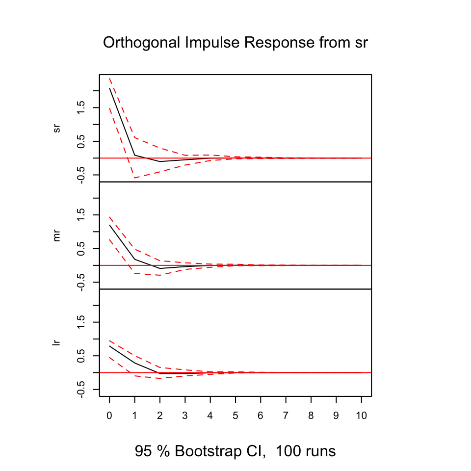
Figure 10.14: Resonses from shocks
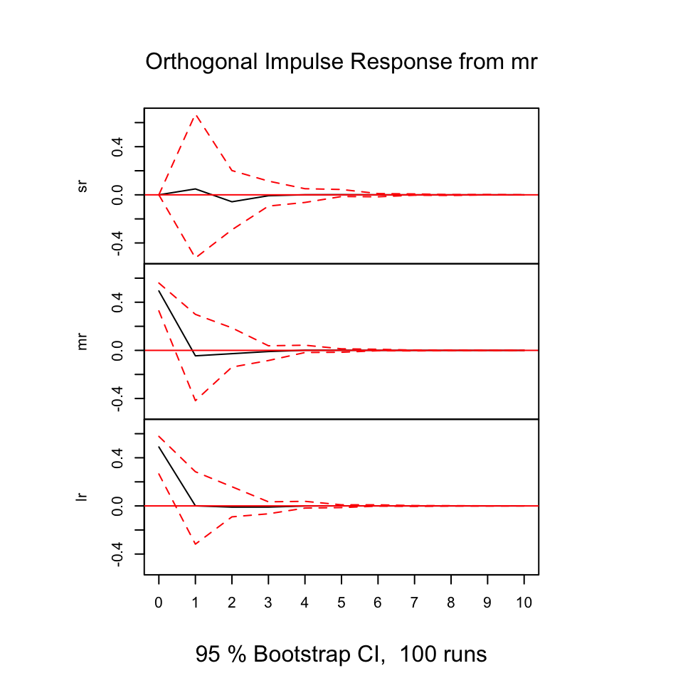
Figure 10.15: Resonses from shocks
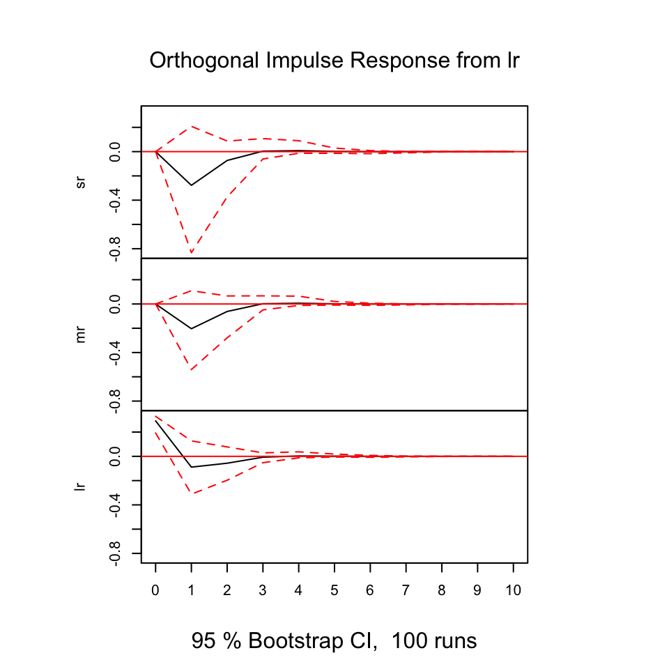
Figure 10.16: Resonses from shocks
10.1.5.1.3.1 Exogenious vs. endogenious
10.1.5.1.4 4. Forecasting with ADL
10.1.5.1.4.1 Step 1 - Data partition
10.1.5.1.4.2 Step 2 - Select the order of VAR
10.1.5.1.4.3 Step 3 - Fit the model + check residuals
10.1.5.1.4.4 Step 4 - Make the forecast
10.1.5.1.4.5 Step 5 - Assessing accuracy
10.1.6 Q7
7. Test for unit roots in each of the series, and determine whether you can obtain a cointegrating relationship. Interpret what your findings suggest.
This was addressed earlier, see the process Q4
rm(list = ls())10.1.7 Case 2
df2 <- read_excel("Data/Exams/Exam2018Case2.xlsx") #Case 2 material10.1.7.1 Q1
dynamic properties
y.badcalls <- ts(df2[,4],frequency = 24)
tsdisplay(y.badcalls)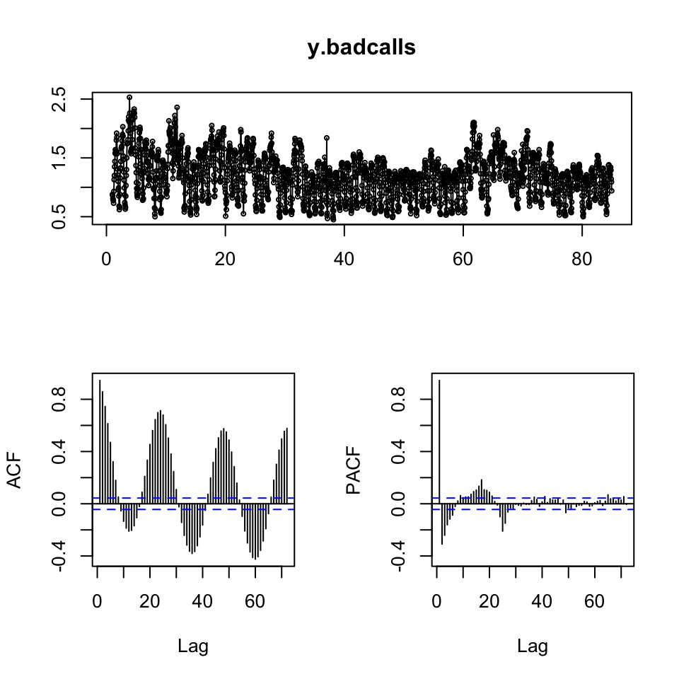
Figure 10.17: Visual inspection
Based on the inspection, we may deduce the following:
- It appears as if we have non stationarity - that can be tested with DW or ADF
- It appears as if there is seasonality - that can be tested with decomposition
Testing for stationarity:
adf.test(y.badcalls)##
## Augmented Dickey-Fuller Test
##
## data: y.badcalls
## Dickey-Fuller = -9.5429, Lag order = 12, p-value = 0.01
## alternative hypothesis: stationaryWe see that the data actually is stationary
A test of decomposing is done in the following question.
On the basis hereon, we are able to deduce that the composition is additive
10.1.7.2 Q2
an appropriate decomposition with explanations on each component
plot(decompose(y.badcalls))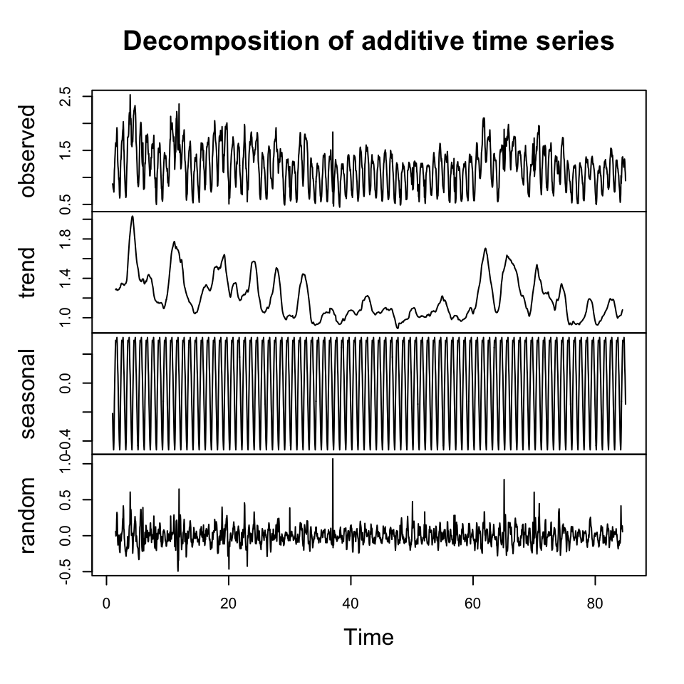
Figure 10.18: Decompisition of Bad Calls
We see that there is no trend in the data, but there is clearly seasons, depending on what hour it is.
We also see no cycles.
10.1.7.3 Q3
linar regression bad calls on the other variables
Checking for stationarity in the explanatory variables
x.pressure <- ts(df2[,2],frequency = 24)
x.windspeed <- ts(df2[,3],frequency = 24)

{print(tsdisplay(x.pressure,lag.max = 500))
print(tsdisplay(x.windspeed,lag.max = 500))}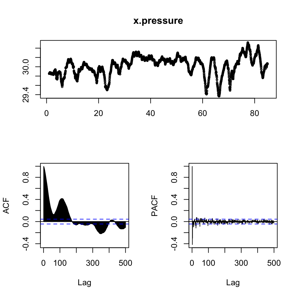
## NULL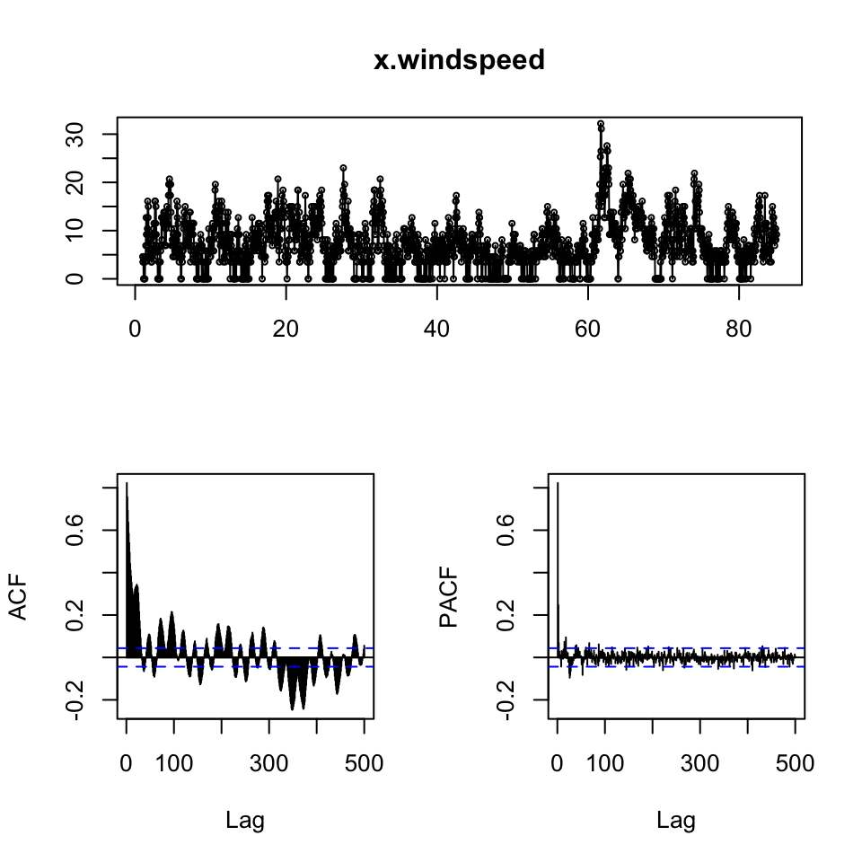
## NULL
{print(adf.test(x.pressure))
print(adf.test(x.windspeed))}
##
## Augmented Dickey-Fuller Test
##
## data: x.pressure
## Dickey-Fuller = -5.4916, Lag order = 12, p-value = 0.01
## alternative hypothesis: stationary
##
##
## Augmented Dickey-Fuller Test
##
## data: x.windspeed
## Dickey-Fuller = -7.2395, Lag order = 12, p-value = 0.01
## alternative hypothesis: stationaryDespite the visual interpretation showing characteristics that appear to be non stationary, the ADF test show overwhelming evidence to reject the null, hence it is fair to assume, that the data is stationer
fit <- lm(y.badcalls ~ x.pressure + x.windspeed)
summary(fit)
##
## Call:
## lm(formula = y.badcalls ~ x.pressure + x.windspeed)
##
## Residuals:
## Min 1Q Median 3Q Max
## -0.70804 -0.20978 0.02901 0.18513 1.07707
##
## Coefficients:
## Estimate Std. Error t value Pr(>|t|)
## (Intercept) 11.486495 1.004297 11.44 <0.0000000000000002 ***
## x.pressure -0.353204 0.033296 -10.61 <0.0000000000000002 ***
## x.windspeed 0.043073 0.001359 31.69 <0.0000000000000002 ***
## ---
## Signif. codes: 0 '***' 0.001 '**' 0.01 '*' 0.05 '.' 0.1 ' ' 1
##
## Residual standard error: 0.2654 on 2013 degrees of freedom
## Multiple R-squared: 0.4803, Adjusted R-squared: 0.4798
## F-statistic: 930.2 on 2 and 2013 DF, p-value: < 0.00000000000000022One could describe this then
10.1.7.4 Q4
a forecast obtained based on an appropriate smoothing method
HW <- HoltWinters(y.badcalls
                  ,beta = FALSE #No trend
                #  ,gamma = TRUE #We have seasons #We want it to calculate the optimal
                  )
HW
## Holt-Winters exponential smoothing without trend and with additive seasonal component.
##
## Call:
## HoltWinters(x = y.badcalls, beta = FALSE)
##
## Smoothing parameters:
## alpha: 0.7433923
## beta : FALSE
## gamma: 0.5407147
##
## Coefficients:
## [,1]
## a 1.0597021787
## s1 -0.1794473089
## s2 -0.2712036049
## s3 -0.3205401341
## s4 -0.3207574608
## s5 -0.3321956847
## s6 -0.2810281488
## s7 -0.2685732309
## s8 -0.1190127729
## s9 -0.0124866501
## s10 0.0978011268
## s11 0.1868982608
## s12 0.2035583267
## s13 0.2205927840
## s14 0.1968599641
## s15 0.1681208212
## s16 0.1624518505
## s17 0.1702619587
## s18 0.1919992681
## s19 0.1975399933
## s20 0.1793936233
## s21 0.1453069693
## s22 0.0598995701
## s23 0.0005213328
## s24 -0.1149900150The model is created with seasonality but not trend hence, Holt Winters smoothing.
The function optimize to the optimal parameters.
forecast(HW,h = 24)## Point Forecast Lo 80 Hi 80 Lo 95 Hi 95
## 85.00000 0.8802549 0.7489360 1.0115738 0.6794199 1.081090
## 85.04167 0.7884986 0.6248691 0.9521280 0.5382489 1.038748
## 85.08333 0.7391620 0.5486245 0.9296996 0.4477600 1.030564
## 85.12500 0.7389447 0.5248548 0.9530347 0.4115224 1.066367
## 85.16667 0.7275065 0.4922100 0.9628030 0.3676515 1.087361
## 85.20833 0.7786740 0.5239302 1.0334178 0.3890770 1.168271
## 85.25000 0.7911289 0.5183207 1.0639372 0.3739047 1.208353
## 85.29167 0.9406894 0.6509407 1.2304381 0.4975570 1.383822
## 85.33333 1.0472155 0.7414636 1.3529675 0.5796083 1.514823
## 85.37500 1.1575033 0.8365450 1.4784616 0.6666400 1.648367
## 85.41667 1.2466004 0.9111244 1.5820765 0.7335342 1.759667
## 85.45833 1.2632605 0.9138695 1.6126516 0.7289130 1.797608
## 85.50000 1.2802950 0.9175222 1.6430677 0.7254819 1.835108
## 85.54167 1.2565621 0.8808841 1.6322402 0.6820121 1.831112
## 85.58333 1.2278230 0.8396684 1.6159776 0.6341918 1.821454
## 85.62500 1.2221540 0.8219117 1.6223963 0.6100362 1.834272
## 85.66667 1.2299641 0.8179886 1.6419397 0.5999019 1.860026
## 85.70833 1.2517014 0.8283177 1.6750852 0.6041919 1.899211
## 85.75000 1.2572422 0.8227496 1.6917347 0.5927432 1.921741
## 85.79167 1.2390958 0.7937715 1.6844201 0.5580311 1.920161
## 85.83333 1.2050091 0.7491104 1.6609079 0.5077722 1.902246
## 85.87500 1.1196017 0.6533683 1.5858352 0.4065593 1.832644
## 85.91667 1.0602235 0.5838796 1.5365675 0.3317183 1.788729
## 85.95833 0.9447122 0.4584679 1.4309565 0.2010657 1.688359We see the above produce point forecasts + confidence intervals.
The following plots the forecast
plot(forecast(HW,h = 24),xlim = c(75,87))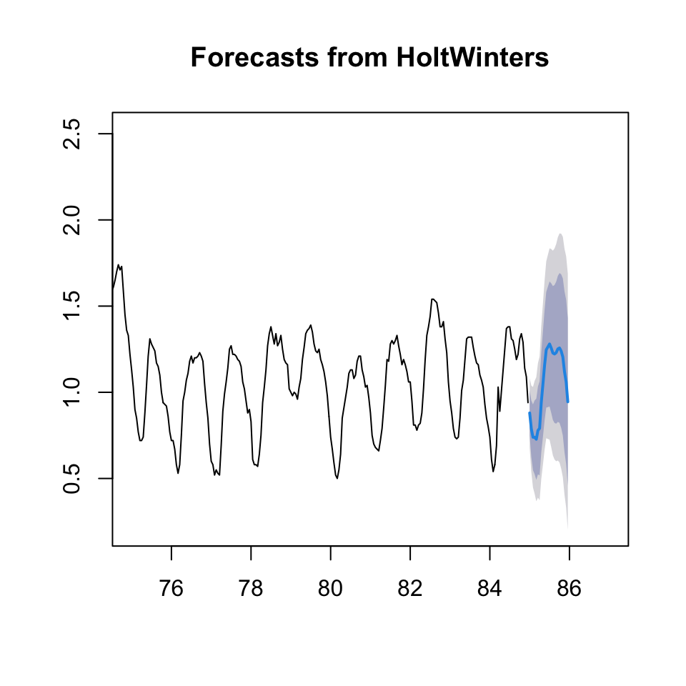
Figure 10.19: HW forecast smoothing
10.1.7.5 Q5
Using ARIMA
arima.bc <- auto.arima(y.badcalls)
forecast(arima.bc,h = 24)
## Point Forecast Lo 80 Hi 80 Lo 95 Hi 95
## 85.00000 0.8952382 0.7597392 1.0307372 0.6880104 1.102466
## 85.04167 0.7915810 0.6146908 0.9684711 0.5210508 1.062111
## 85.08333 0.6938403 0.4895408 0.8981398 0.3813912 1.006289
## 85.12500 0.6974756 0.4730226 0.9219285 0.3542044 1.040747
## 85.16667 0.7282253 0.4884601 0.9679905 0.3615361 1.094915
## 85.20833 0.8758832 0.6232167 1.1285497 0.4894632 1.262303
## 85.25000 0.8537510 0.5902471 1.1172550 0.4507565 1.256746
## 85.29167 0.9649759 0.6923134 1.2376385 0.5479745 1.381977
## 85.33333 1.0753636 0.7949200 1.3558072 0.6464621 1.504265
## 85.37500 1.2120036 0.9249268 1.4990804 0.7729575 1.651050
## 85.41667 1.3387255 1.0459649 1.6314861 0.8909867 1.786464
## 85.45833 1.3620451 1.0643968 1.6596933 0.9068313 1.817259
## 85.50000 1.3819627 1.0800996 1.6838259 0.9203029 1.843623
## 85.54167 1.3872987 1.0817924 1.6928050 0.9200672 1.854530
## 85.58333 1.3670515 1.0583905 1.6757125 0.8949952 1.839108
## 85.62500 1.3303459 1.0189487 1.6417430 0.8541050 1.806587
## 85.66667 1.2923932 0.9786197 1.6061666 0.8125181 1.772268
## 85.70833 1.2818309 0.9659914 1.5976704 0.7987960 1.764866
## 85.75000 1.2748361 0.9571985 1.5924738 0.7890513 1.760621
## 85.79167 1.2786251 0.9594213 1.5978289 0.7904451 1.766805
## 85.83333 1.2578344 0.9372655 1.5784033 0.7675666 1.748102
## 85.87500 1.1380432 0.8162837 1.4598027 0.6459545 1.630132
## 85.91667 1.0700041 0.7472057 1.3928025 0.5763266 1.563682
## 85.95833 0.9407264 0.6170210 1.2644318 0.4456617 1.435791plot(forecast(arima.bc,h = 24),xlim = c(75,87))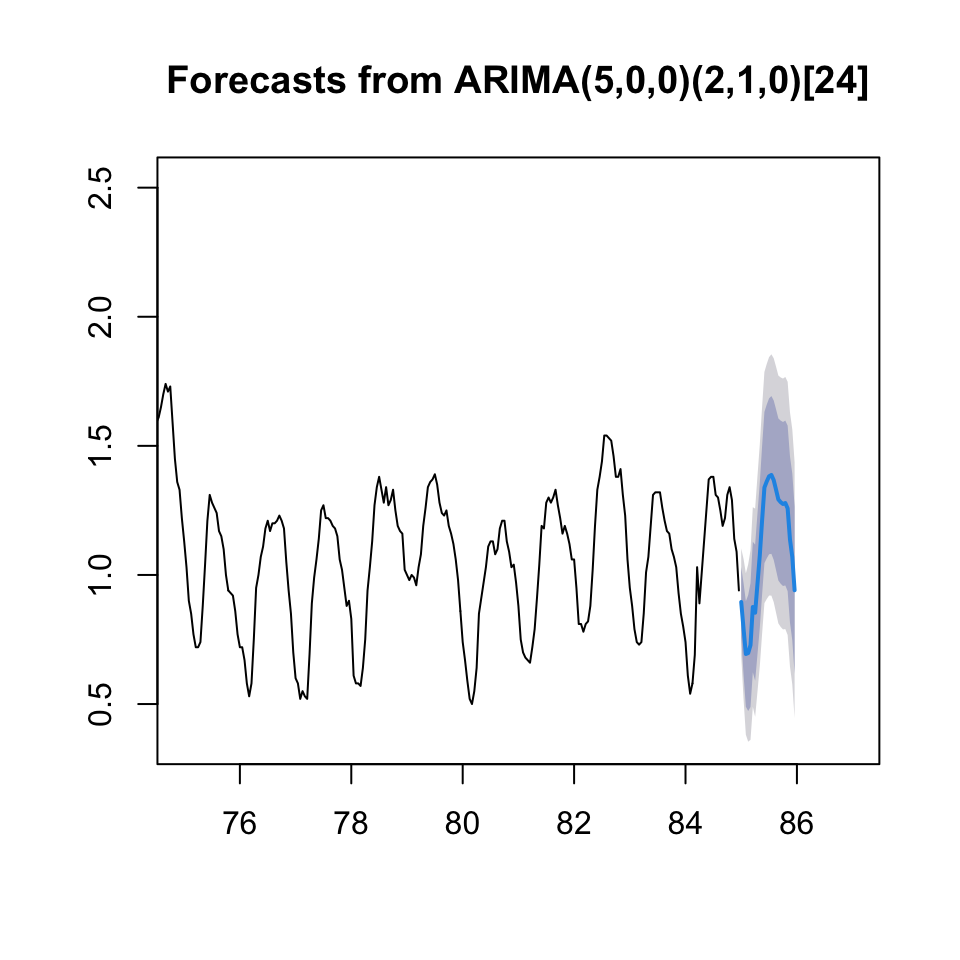
10.1.7.6 Q6
a forecast combination of the two previously chosen methods and their evaluations
Let us use the HoltWinters smoothing and the arima from q4 and q5.
First we must find out if it is fair to assume, that the models perform equally good. That can be done with Diebold-Mariano test. Where H0: is that the MSE’s are not significantly far from each other.
dm.test(e1 = resid(HW)
        ,e2 = resid(arima.bc)[25:2016]
        ,alternative = "two.sided" #Default, but shown for pedogical reasons. meaning that H1 is a two sided test
        )
##
## Diebold-Mariano Test
##
## data: resid(HW)resid(arima.bc)[25:2016]
## DM = -1.7642, Forecast horizon = 1, Loss function power = 2, p-value =
## 0.07786
## alternative hypothesis: two.sidedWe are not able to reject the null hypothesis, hence the accuracies can be assumed to be the same, hence equally good models.
10.1.7.6.1 Combined model
Now we can make the combined model, this can be done with two approaches:
- Nelson
- Granger-Ramanathan
comb.df <- as.data.frame(cbind(as.matrix(y.badcalls[25:2016])
                               ,as.vector(HW$fitted[,1])
                               ,as.vector(arima.bc$fitted[25:2016])))
names(comb.df) <- c("y.badcalls","x.HW","x.arima")

combfit <- lm(y.badcalls ~ x.HW + x.arima
              ,data = comb.df)

summary(combfit) #the coefficients in the regression will give you the weights
##
## Call:
## lm(formula = y.badcalls ~ x.HW + x.arima, data = comb.df)
##
## Residuals:
## Min 1Q Median 3Q Max
## -0.91363 -0.04814 -0.00527 0.04445 1.19600
##
## Coefficients:
## Estimate Std. Error t value Pr(>|t|)
## (Intercept) 0.060838 0.007844 7.756 0.0000000000000139 ***
## x.HW 0.693959 0.042933 16.164 < 0.0000000000000002 ***
## x.arima 0.255147 0.044773 5.699 0.0000000138793768 ***
## ---
## Signif. codes: 0 '***' 0.001 '**' 0.01 '*' 0.05 '.' 0.1 ' ' 1
##
## Residual standard error: 0.09884 on 1989 degrees of freedom
## Multiple R-squared: 0.9279, Adjusted R-squared: 0.9278
## F-statistic: 1.28e+04 on 2 and 1989 DF, p-value: < 0.00000000000000022combfcast <- ts(combfit$fitted.values, frequency = 24)
plot(combfcast)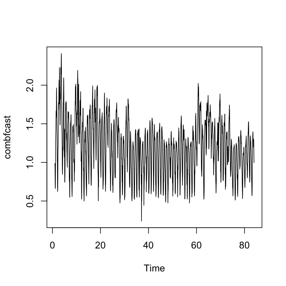
accuracy(combfcast,x = comb.df$y.badcalls)## ME RMSE MAE MPE MAPE
## Test set -0.000000000000000001959061 0.09877032 0.06512255 -0.7175288 5.916592