4.4 Exercises
This section contain exercises, hence the methods applied on data
4.4.1 p. 92 HW Problem 8
4.4.1.1 Moving Averages
Yana has shown a loop for doing MA, that will be tested, hence this section contain two subsections:
- Regular MA, as it was done during lectures
- MA with loop.
4.4.1.1.1 Regular MA
df <- read_excel("Data/Week45/prob8p92HW.xlsx")
yt <- ts(df) #Rename and define as time series
ts.plot(yt) #We can plot the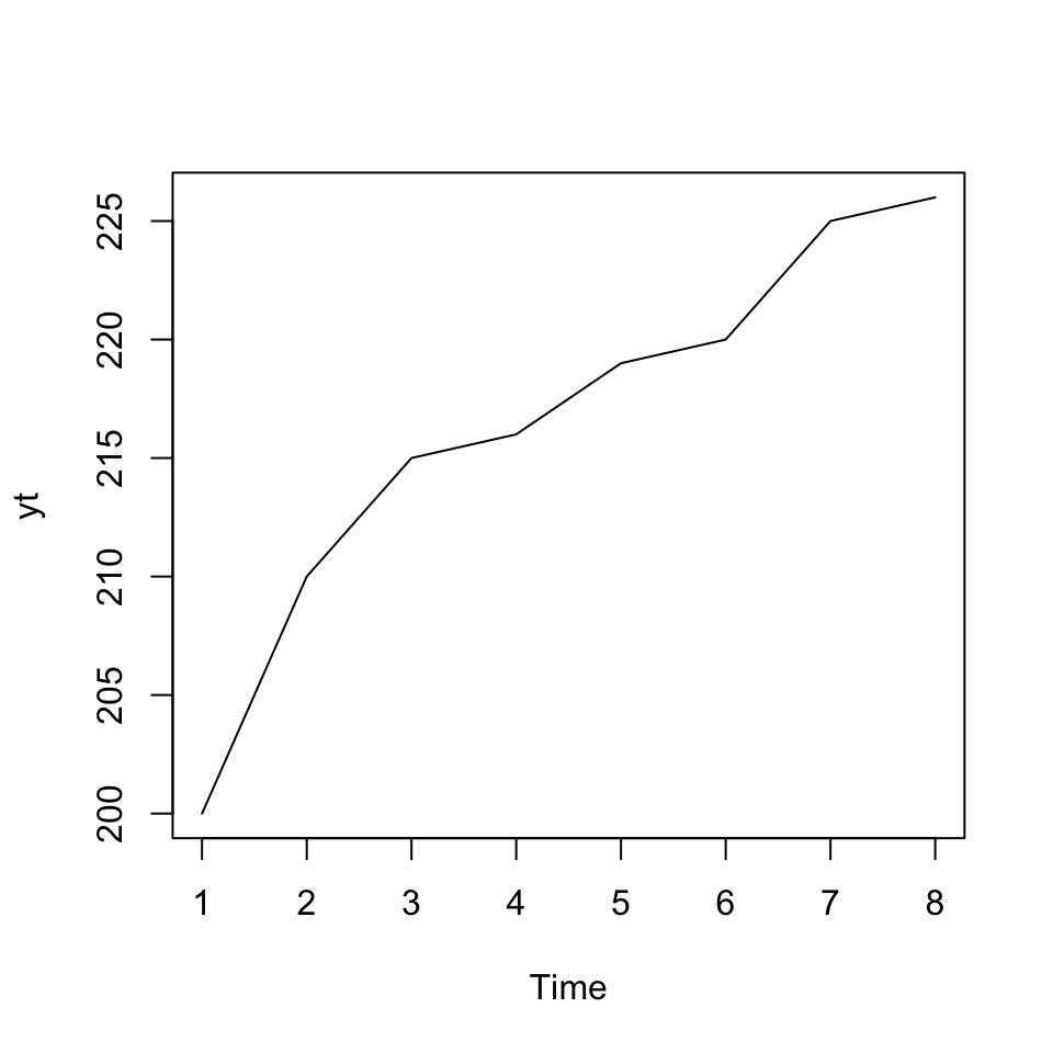
We see that there is a trend in the data.
We can calculate the five period moving average by:
yt5c <- ma(yt #The time series
           ,order = 5 #Amount of periods to be evaluated
           ,centre = TRUE #We want the center value of the MA
           )
yt5c
## Time Series:
## Start = 1
## End = 8
## Frequency = 1
## [,1]
## [1,] NA
## [2,] NA
## [3,] 212.0
## [4,] 216.0
## [5,] 219.0
## [6,] 221.2
## [7,] NA
## [8,] NAHence we are able to produce moving averages based on the data. Notice, that the most recent MA is the prediction, hence being \(\hat{Y}_{t+1}\).
One could extend this, by adding this value to the time series and then calculate MA for the period hereafter. We see that the output of the table above is somewhat misleading, as the most recent MA predictinos, are not positioned in the end, but instead where the center actually is.
This problem is solvable using filter(). See the following chunk
k <- 5 #specify the order of the moving average
c <- rep (1/k,k) #remember that simple average is a weighted average with equal weights,
                #you need to specify weights for the filter command to work
yt5<- filter(yt, c, sides = 1)
ts.plot(yt5)# "Plotting the MA's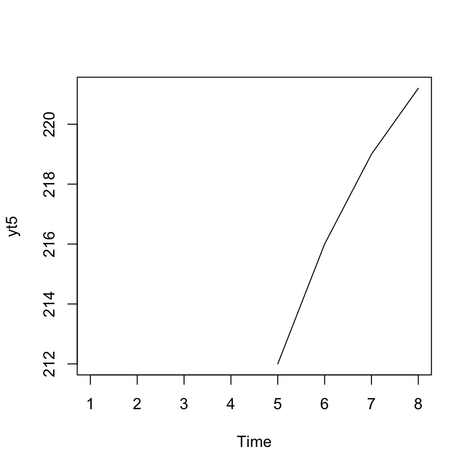
Figure 4.4: 5k Moving Average
yt5 #The updated vector of MA's## Time Series:
## Start = 1
## End = 8
## Frequency = 1
## [,1]
## [1,] NA
## [2,] NA
## [3,] NA
## [4,] NA
## [5,] 212.0
## [6,] 216.0
## [7,] 219.0
## [8,] 221.2This we see, that scores are moved to the end, so even though it is the center of the MA, it is now presented as recent values.
For simple moving averages, one may do it in excel, it may be easier and quicker.
4.4.1.1.2 MA using loop
#Define the input data
#dy.ltn <- dy.ltn

#Forecasting with a simple MA of order k
k <- 5
l <- length(yt) #number of available data points

#adding extra rows, as many as periods ahead want to forecast
h <-18
y <- yt

#generating space to save the forecasts
for (i in 1:h){
  y <- c(y, 0)
}

#t(t(y)) #One could show the result

#calculating the forecast values
for (j in (l+1):(l+h)){ #Notice,
  print(j)
  a<-j-k
  b<-j-1
  x <-y[a:b]
  y[j] <- mean(x)
}
## [1] 9
## [1] 10
## [1] 11
## [1] 12
## [1] 13
## [1] 14
## [1] 15
## [1] 16
## [1] 17
## [1] 18
## [1] 19
## [1] 20
## [1] 21
## [1] 22
## [1] 23
## [1] 24
## [1] 25
## [1] 26
result1 <- t(t(y)) #One could show the result


#Plotting
plot(y,type = 'l',main = "MA, k = 5")
abline(v = l,col = "red")
grid(col = "lightgrey")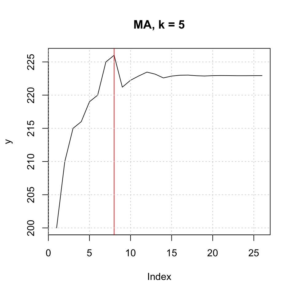
4.4.1.2 Exponential moving averages + Holts and Winters
Simple exponential smoothing
Where;
- alpha is the smoothing parameter,
- beta tells you if you should account for a trend or not,
- gamma is responsible for the presence of a seasonal component in the model
fit <- HoltWinters(yt
                   ,alpha = 0.4
                   ,beta = FALSE
                   ,gamma = FALSE)
plot(fit,xlim = c(1,nrow(df))) + grid(col = "lightgrey")
## integer(0)legend("topleft",c("Observed","Fitted"),lty = 1,col = c(1:2))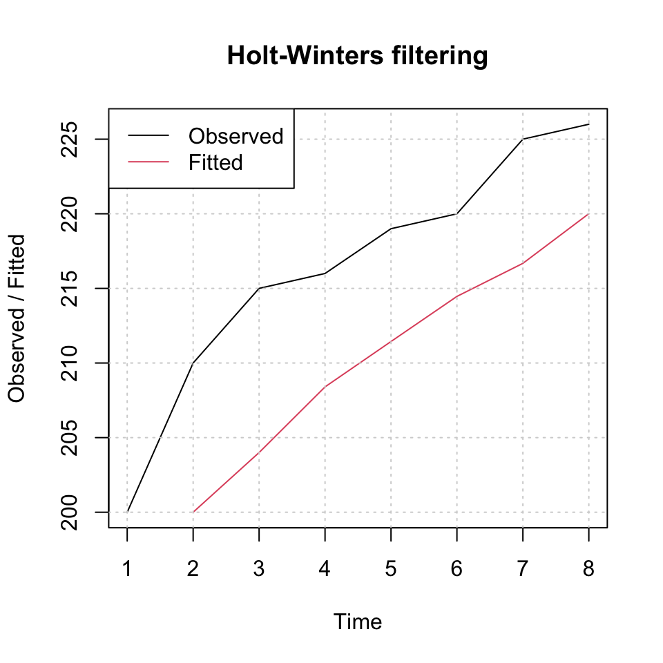
Figure 4.5: Exponential Smoothing
Hence we see the smoothed values, where the higher alpha, the more will the fitted line track the changes in the observations.
We can now plot the forecast values:
plot(forecast(fit),xlim = c(1,nrow(df)+10))# + grid(col = "lightgrey")
legend("topleft",c("Observed","Forecast"),lty = 1,col = c("Black","Blue"))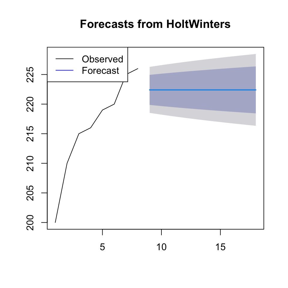
Figure 4.6: Forecast Exponential Smoothing
One see the confidence intervals of the forecast widening as we get further away from the actual values.
Now one may assess the accuracy:
accuracy(forecast(fit))## ME RMSE MAE MPE MAPE MASE ACF1
## Training set 8.001509 8.209102 8.001509 3.673623 3.673623 2.154252 0.1962194One see an RMSE of 8.2. Hence one could compare it with an exponential smoothing, which is more sensitive to the observations.
fit0.6 <- HoltWinters(yt
                   ,alpha = 0.6 #Changed
                   ,beta = FALSE
                   ,gamma = FALSE)
accuracy(forecast(fit0.6))
## ME RMSE MAE MPE MAPE MASE ACF1
## Training set 5.860023 6.373698 5.860023 2.700235 2.700235 1.577698 0.264614Where we see an RMSE of 6.37, hence lower than the initial test.
Holt’s exponential smoothing
exponential smoothing when a trend component is present: beta = TRUE
{fit3 <- HoltWinters(yt
                    ,alpha = 0.6
                    ,beta = TRUE
                    ,gamma = FALSE)
plot(forecast(fit3))
accuracy(forecast(fit3))}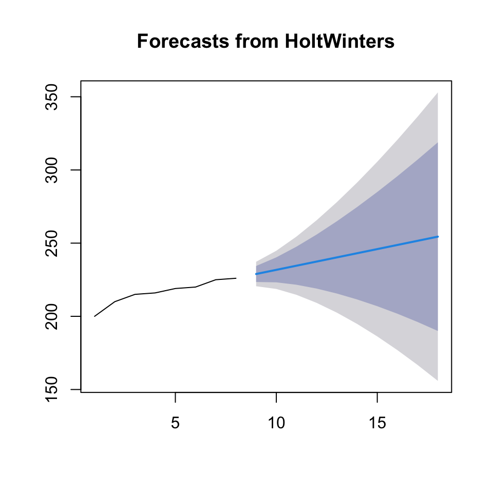
Figure 4.7: Holt’s Exponential Smoothing
##                     ME     RMSE      MAE        MPE     MAPE     MASE      ACF1
## Training set -1.990133 4.369207 3.451467 -0.9324372 1.581919 0.929241 0.4352197
We see that the RMSE is even lower (4.37). Which is expected, as Holt’s exponential smoothing accounts for trend.
Winter’s Exponential Smoothing
Which accounts for trend and seasonality
in order to make it work one needs to define the frequency of your seasonal component, when specifying the ts data
{yt <- ts(df
         ,frequency = 4) # let's assume we suspect a quarterly pattern
fit4 <- HoltWinters(yt, alpha=0.6, beta=TRUE, gamma=TRUE)
plot(forecast(fit4))
accuracy(forecast(fit4))} # experiment with seasonality frequency to see if you can get any lower in MSE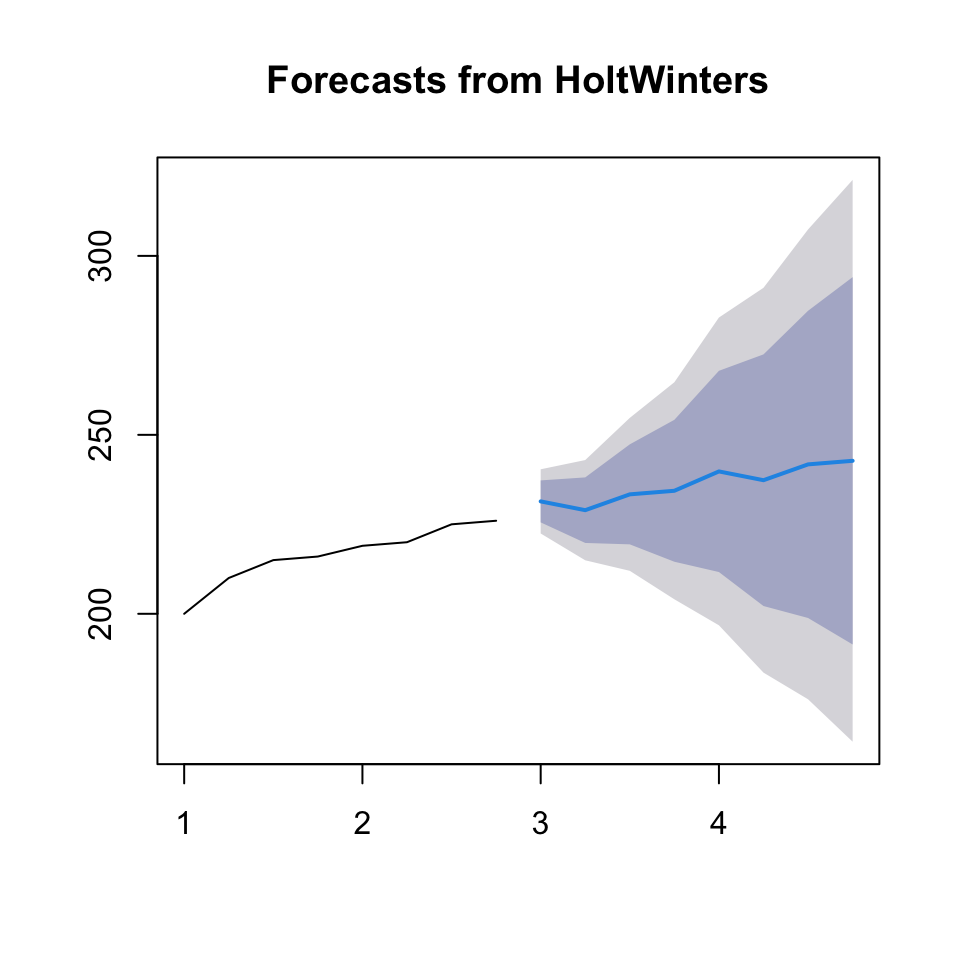
##                     ME     RMSE     MAE        MPE    MAPE      MASE
## Training set -0.310075 3.973148 3.34445 -0.1227802 1.50834 0.2730163
##                     ACF1
## Training set 0.009251985
We see that the RMSE is even lower (3.97), hence Winters Exponential Smoothing appear to be the best model for prediction.
4.4.2 p. 93 HW Problem 9-10
Basically just another example of the exercise above.
4.4.3 CO2 and Sales Data
Not done again. Do if time allows.
4.4.4 Case 6 oo. 108-111 HW
Not done again. Do if time allows.