8.4 Exercises
8.4.1 Dairy Data
Loading the data. We have yearly data and select employment data.
df <- read_xls("Data/Week49/dairydata.xls")
y <- df$emp %>% log() %>% ts() #Frequency is by default 1, that is applied, as we have yearly data
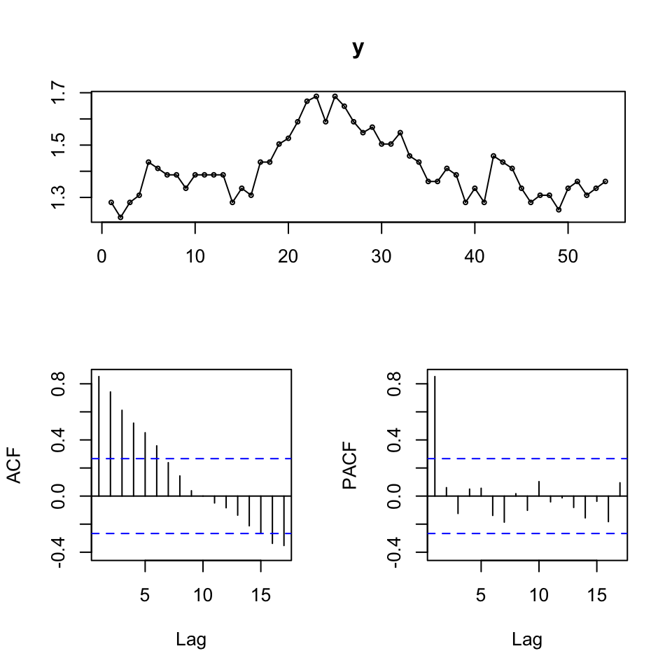
tsdisplay(y)
Figure 8.1: Visual interptration
Notice that we take log, that is done to smooth out extreme values, and make the data more normal.
Based on the figure, we are able to deduce:
- The ts does not appear to show stationarity, that is to be further inspected in 8.4.1.1
- That there is clearly a trend
- The acf does not imply, that the data show autocorrelation
8.4.1.1 Unit Root testing - Augmented Dickey-Fuller (ADF)
We aim to find out if there is statistical evidence for unit roots (nonstationarity), that is done with the adf.
First we make ADF on the time series, hence \(y_t\)
adf.test(y)##
## Augmented Dickey-Fuller Test
##
## data: y
## Dickey-Fuller = -1.9669, Lag order = 3, p-value = 0.5879
## alternative hypothesis: stationaryNote, the null hypothesis is that the data show nonstationarity
Based on the ADF on the log of the data, we are not able to reject the null hypothesis, hence the time series does not show stationarity, that is as expected, as we saw from the ts plot.
We can take the first order difference to see if we can get rid of the nonstationarity.
dy <- diff(y,lag = 1) #lag 1 is default, but shown for explanatory reasons
adf.test(dy) #Rejecting the null, so can claim stationarity of the differenced series
##
## Augmented Dickey-Fuller Test
##
## data: dy
## Dickey-Fuller = -3.8763, Lag order = 3, p-value = 0.0216
## alternative hypothesis: stationaryNow we are able to reject the null hypothesis. We can then look at this visually.
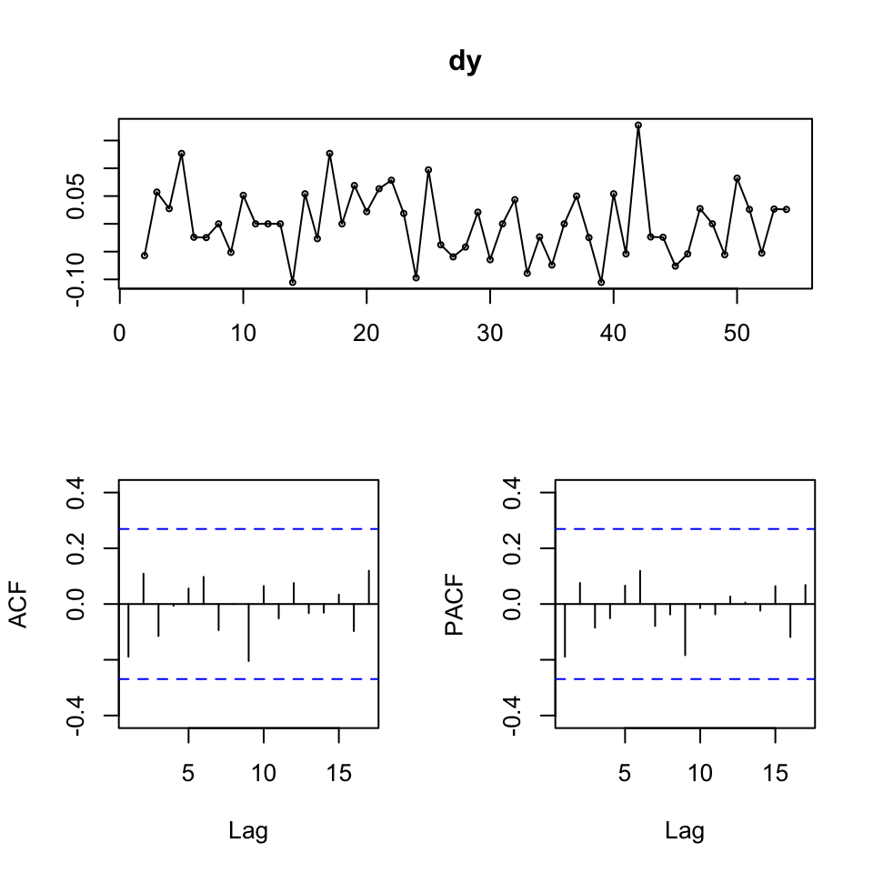
tsdisplay(dy)
Figure 8.2: tsdisplay dy
This just confirms the hypothesis test.
Conclusion
With ADF, we are able to make a statistical test for stationarity, hence it is able to support the visual interpretation.
8.4.1.2 Cointegration
Now we extend the data and introduce another variable, production worker hours, hence \(x_t\).
As with the y variable, the data is annually and we take the log of the data. As with y, we must check for stationarity, hence:
x <- ts(log(df$prodh)) #production worker hours
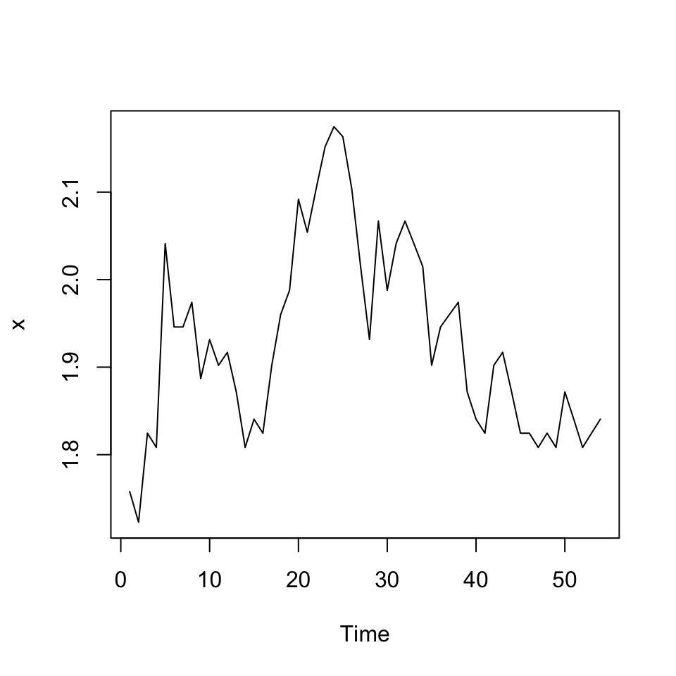
plot(x)
The data does not look stationary, lets do an ADF, to make a statistical test for this.
adf.test(x)##
## Augmented Dickey-Fuller Test
##
## data: x
## Dickey-Fuller = -2.4693, Lag order = 3, p-value = 0.3855
## alternative hypothesis: stationaryWe are not able to reject the null hypothesis, hence x being non stationarity (i.e. non stationary in levels). Lets do first order differencing and check ADF for that:
adf.test(diff(x))##
## Augmented Dickey-Fuller Test
##
## data: diff(x)
## Dickey-Fuller = -5.1438, Lag order = 3, p-value = 0.01
## alternative hypothesis: stationaryWe see that we are able to reject H0.
8.4.1.2.1 Graphical inspection of the data
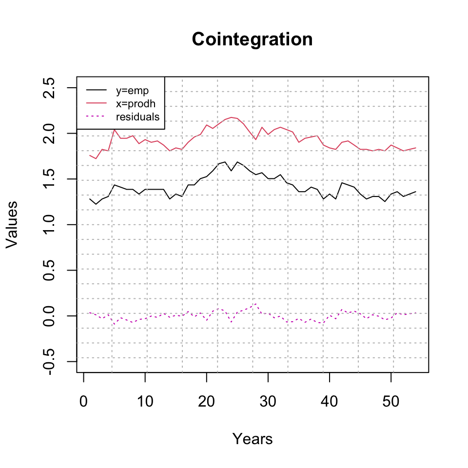
To show this graphically, we can represent the following.
plot(y,col = 1,ylim = c(-0.5,2.5),main = "Cointegration",xlab = "Years",ylab = "Values") +
  lines(x,col = 2) +
  lines(residuals(lm(y~x)),col = 6,lty = 3) +
  grid(col = "grey",nx = 10,ny = 20)
## integer(0)legend(x = "topleft",legend = c("y=emp","x=prodh","residuals"),lty = c(1,1,3),col = c(1,2,6),cex = 0.7)
Figure 8.3: Representation of cointegration
We see that the time-series’ (which are not difference) are not stationary and the perfectly fits each other. Let us assume, that these are not spurously related, then they are in fact cointegrated.
When a regression is run on the two variables, we see that the residuals show stationarity, hence that is a good indication of cointegration.
This can be further explored with the following two procedures:
8.4.1.2.2 Test for cointegration
- Statistical test - Phillips-Ouliaris test (2-step EG test), whith H0: no cointegration This is supposed to be the better option, as it uses the correct distributions, that was just briefly mentioned during class
- Manual process, consisting of:
- Fitting y on x
- Checking the residuals for unit roots (stationarity) using ADF.
The following does both:
Option 1 - Phillips-Ouliaris test
# Combining the two vectors x and y
z <- ts(cbind(x,y))

po.test(z) #Note, this is the 2-step EG test
##
## Phillips-Ouliaris Cointegration Test
##
## data: z
## Phillips-Ouliaris demeaned = -33.724, Truncation lag parameter = 0,
## p-value = 0.01We have H0: no cointegration.
We are able to reject the null, hence it is fair to assume that there is cointegration between the two variables.
Option 2 - Manual process
fit <- lm(y~x) #Running an OLS of y on x
adf.test(x = resid(fit)) #Testing if the residuals from the estimated model contain a unit root.
##
## Augmented Dickey-Fuller Test
##
## data: resid(fit)
## Dickey-Fuller = -2.7005, Lag order = 3, p-value = 0.2924
## alternative hypothesis: stationaryADF H0: x = non stationary
We see that this does in fact not show stationarity, which contradicts with the PO test.
Although the adf.test is not always applying the correct distributions, hence it may not align with the PO test, which is what we see in this.